plotgardener uses a coordinate-based plotting system to
define the size and location of plots. This system makes the plotting
process intuitive and absolute, meaning that plots cannot be squished
and stretched based on their relative sizes. This also allows
for precise control of the size of each visualization and the location
of all plots, annotations, and text.
All plotgardener page functions begin with the
page prefix.
Users can create a page in their preferred size and unit of
measurement using pageCreate(). Within this function the
user can also set gridlines in the vertical and horizontal directions
with xgrid and ygrid, respectively. By default
these values are set to 0.5 of the unit. In the following example we
demonstrate creating a standard 8.5 x 11 inch page:
pageCreate(width = 8.5, height = 11, default.units = "inches")
Or we could create a smaller sized page in a different set of units with different gridlines:
pageCreate(width = 8, height = 8, xgrid = 1, ygrid = 1, default.units = "cm")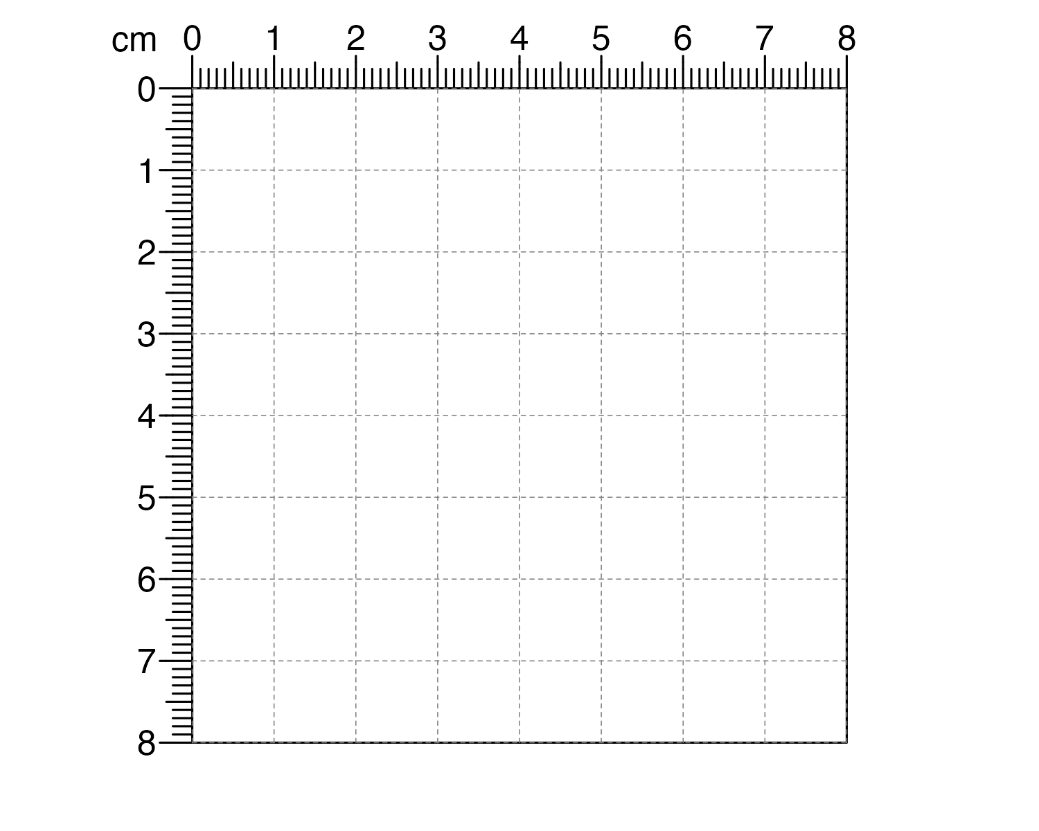
We could turn off gridlines entirely by setting xgrid
and ygrid to 0:
pageCreate(
    width = 3, height = 3, xgrid = 0, ygrid = 0,
    default.units = "inches"
)
If we want more specific gridlines on our page, we can use the
pageGuideHorizontal() and pageGuideVertical()
functions:
pageCreate(width = 3, height = 3, default.units = "inches")
## Add a horizontal guide at y = 2.25 inches
pageGuideHorizontal(y = 2.25, default.units = "inches")
## Add a vertical guide at x = 0.75 inches
pageGuideVertical(x = 0.75, default.units = "inches")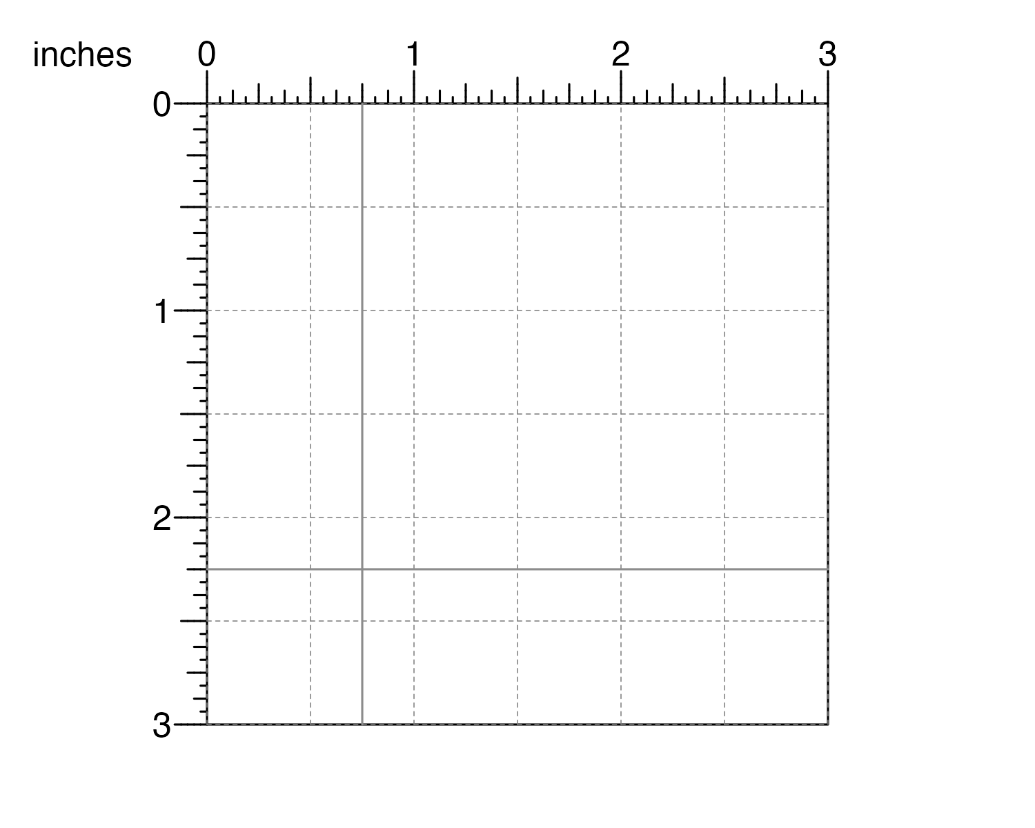
We can also remove all guidelines from the plot once we are finished
using guides by using the pageGuideHide() function:
## Create page
pageCreate(width = 3, height = 3, default.units = "inches")
## Remove guides
pageGuideHide()
Coordinate systems and units
plotgardener is compatible with numerous coordinate
systems, which are flexible enough to be used in combination. Brief
descriptions of the most commonly used plotgardener
coordinate systems are as follows:
| Coordinate System | Description |
|---|---|
| “npc” | Normalized Parent Coordinates. Treats the bottom-left corner of the plotting region as the location (0,0) and the top-right corner as (1,1). |
| “snpc” | Squared Normalized Parent Coordiantes. Placements and sizes are expressed as a proportion of the smaller of the width and height of the plotting region. |
| “native” | Placements and sizes are relative to the x- and y-scales of the plotting region. |
| “inches” | Placements and sizes are in terms of physical inches. |
| “cm” | Placements and sizes are in terms of physical centimeters. |
| “mm” | Placements and sizes are in terms of physical millimeters. |
| “points” | Placements and sizes are in terms of physical points. There are 72.27 points per inch. |
We can set the page in one coordinate system, but then
place and arrange our plots using other coordinate systems. For example,
we can set our page as 3 x 3 inches:
pageCreate(width = 3, height = 3, default.units = "inches")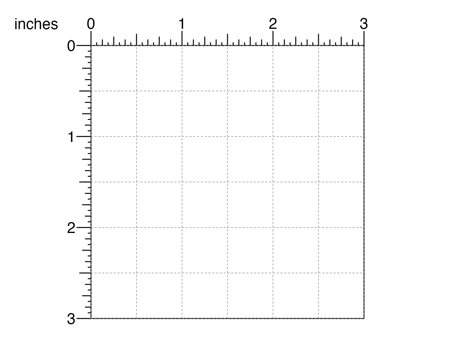
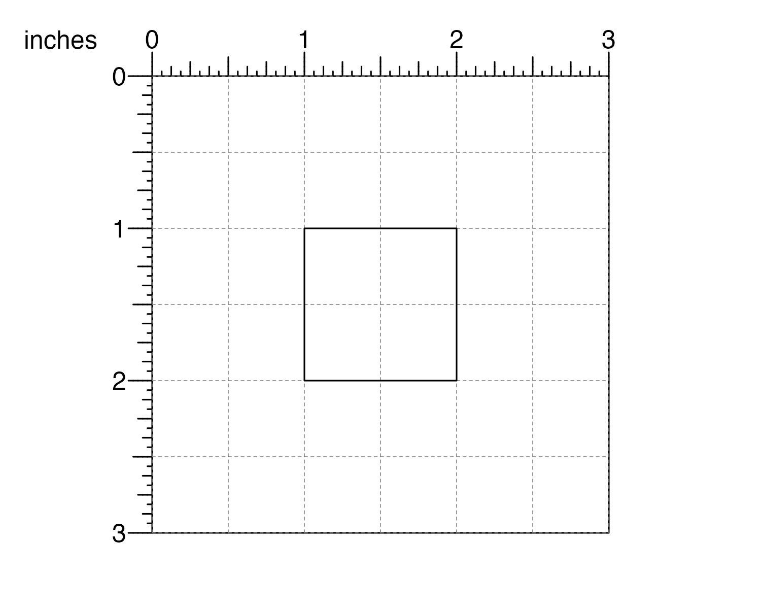
But we can then switch to npc coordinates to plot
something in the center of the page at (0.5, 0.5) npc. The
unit() function allows us to easily specify x,
y, width, and height in
combinations of different units in one plotting function call.
plotRect(
    x = unit(0.5, "npc"), y = unit(0.5, "npc"), width = 1, height = 1,
    default.units = "inches"
)
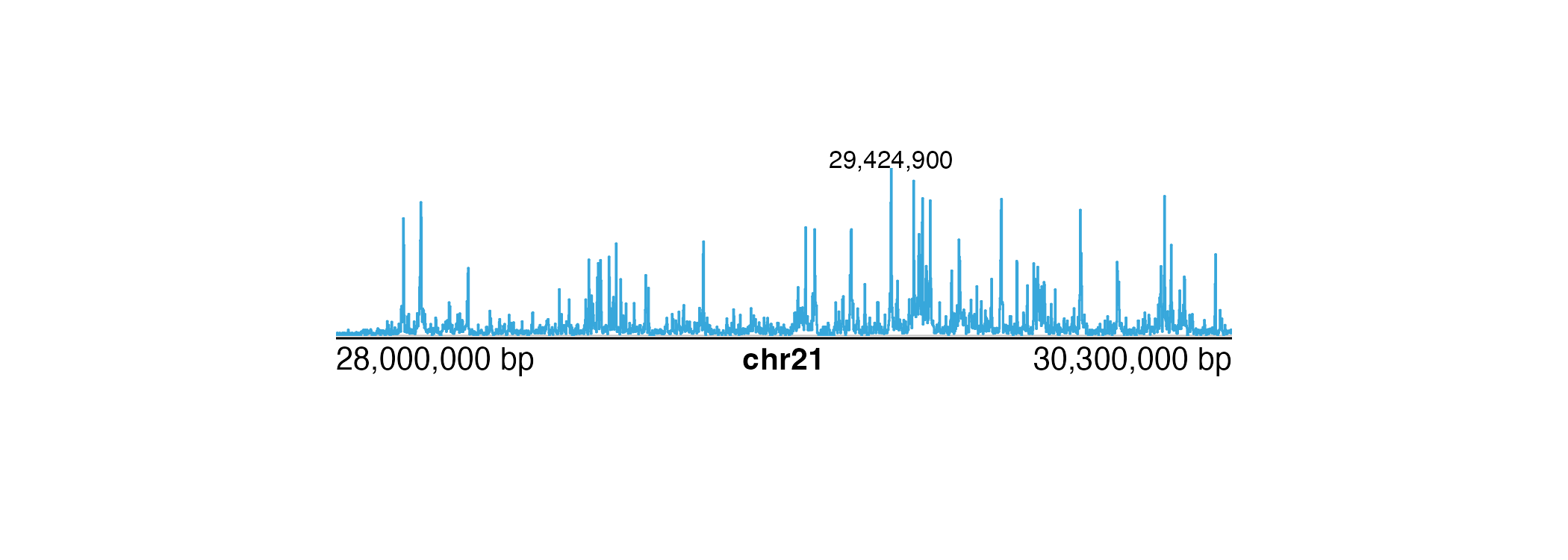
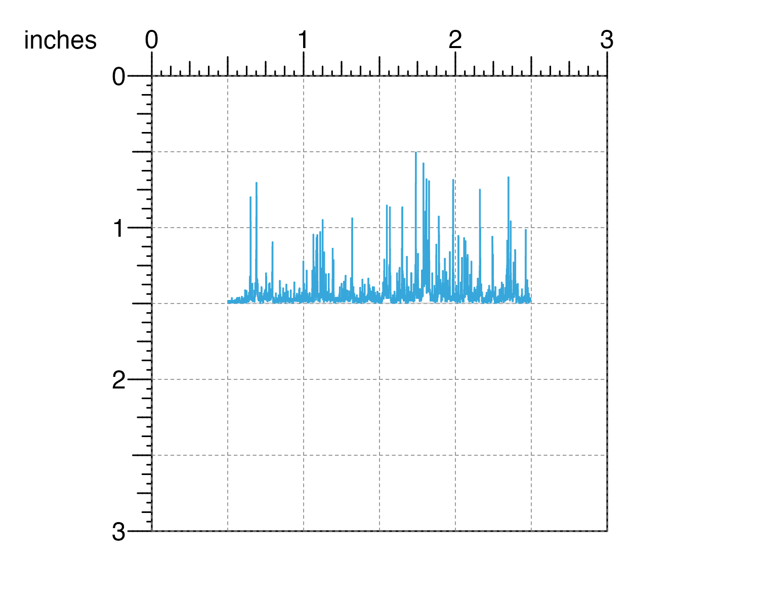
The native coordinate system is particularly useful
for annotation functions that can plot relative to the genomic scales of
a plot. For example, we can use annoText() to annotate some
text at a specific genomic location in a plot:
pageCreate(
    width = 5, height = 1.5, default.units = "inches",
    showGuides = FALSE, xgrid = 0, ygrid = 0
)

library(plotgardenerData)
data("IMR90_ChIP_H3K27ac_signal")
signalPlot <- plotSignal(
    data = IMR90_ChIP_H3K27ac_signal,
    chrom = "chr21", chromstart = 28000000, chromend = 30300000,
    assembly = "hg19",
    x = 0.5, y = 0.25, width = 4, height = 0.75, default.units = "inches"
)
annoGenomeLabel(plot = signalPlot, x = 0.5, y = 1.01)

## Annotate text at average x-coordinate of data peak
peakScore <- IMR90_ChIP_H3K27ac_signal[which(
    IMR90_ChIP_H3K27ac_signal$score == max(IMR90_ChIP_H3K27ac_signal$score)
), ]
peakPos <- round((min(peakScore$start) + max(peakScore$end)) * 0.5)
annoText(
    plot = signalPlot, label = format(peakPos, big.mark = ","), fontsize = 8,
    x = unit(peakPos, "native"), y = unit(1, "npc"),
    just = "bottom"
)
Working with plot objects
In plotgardener all plot objects are boxes, with
user-defined positions and sizes. All plot objects can be placed on a
page using the placement arguments (e.g. x,
y, width, height,
just, default.units, …). The page
sets the origin of the plot at the top left corner of the page. By
default, the x and y arguments place the
top-left corner of a plot in the specified position on the
page while the width and height
arguments define the size of the plot.
For example, if users want the top-left corner of their plot to be 0.5 inches down from the top of the page and 0.5 inches from the left…
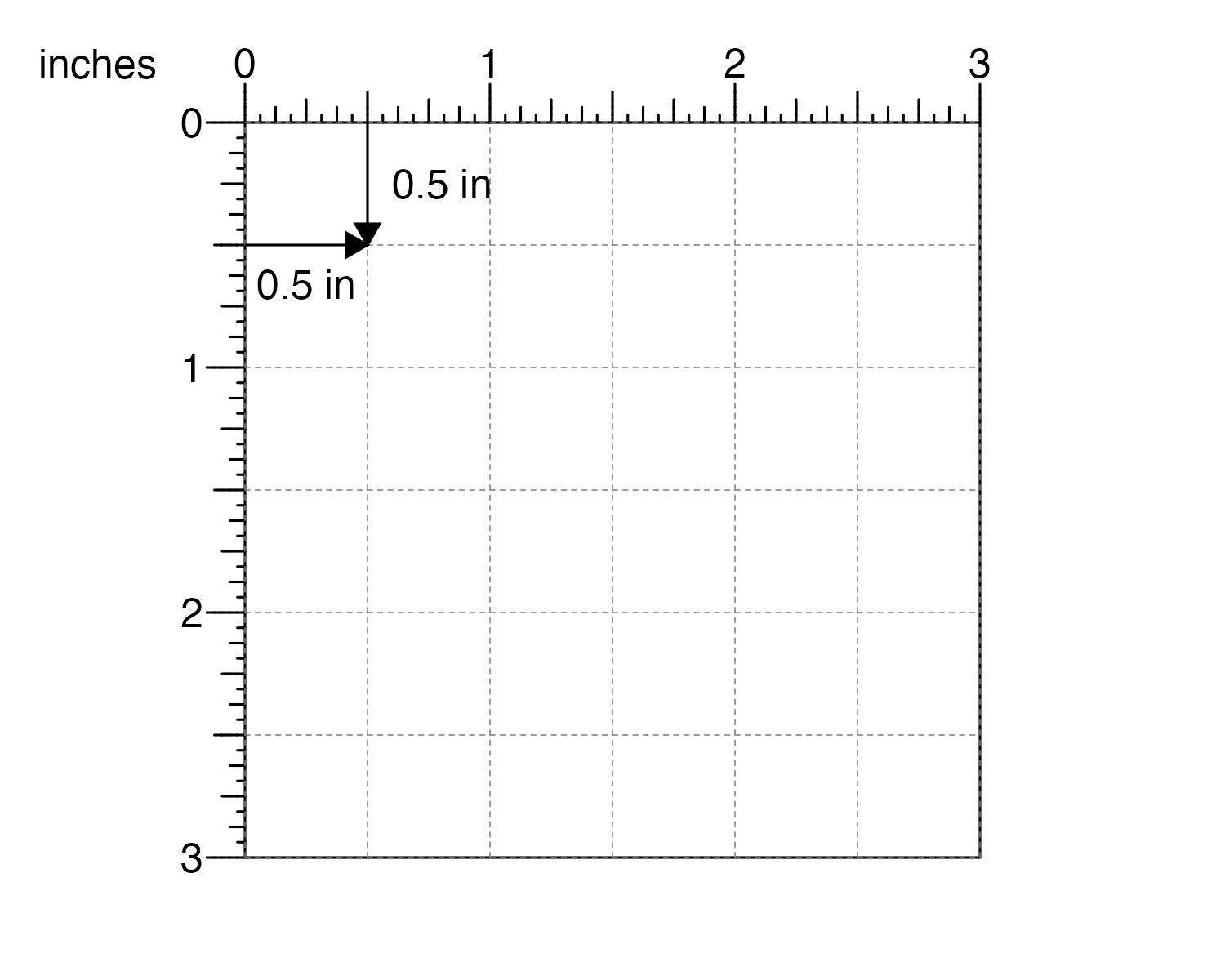
and the plot to be 2 inches wide and 1 inch tall…
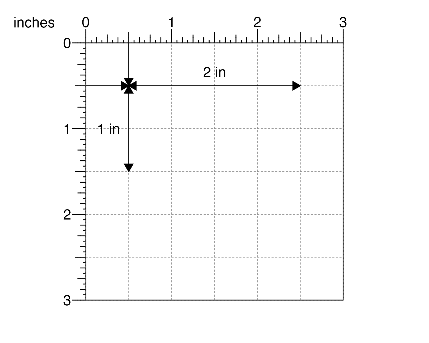
plotgardener can make the plot with these exact
dimensions:
## Create page
pageCreate(width = 3, height = 3, default.units = "inches")

## Plot rectangle
plotRect(
    x = 0.5, y = 0.5, width = 2, height = 1,
    just = c("left", "top"), default.units = "inches"
)
plotgardener also provides the helper function
pagePlotPlace() for placing plot objects that have been
previously defined:
## Load data
library(plotgardenerData)
data("IMR90_ChIP_H3K27ac_signal")

## Create page
pageCreate(width = 3, height = 3, default.units = "inches")

## Define signal plot
signalPlot <- plotSignal(
    data = IMR90_ChIP_H3K27ac_signal,
    chrom = "chr21", chromstart = 28000000, chromend = 30300000,
    assembly = "hg19",
    draw = FALSE
)

## Place plot on page
pagePlotPlace(
    plot = signalPlot,
    x = 0.5, y = 0.5, width = 2, height = 1,
    just = c("left", "top"), default.units = "inches"
)
and pagePlotRemove() for removing plots from a page:
# Load data
library(plotgardenerData)
data("IMR90_ChIP_H3K27ac_signal")

## Create page
pageCreate(width = 3, height = 3, default.units = "inches")

## Plot and place signal plot
signalPlot <- plotSignal(
    data = IMR90_ChIP_H3K27ac_signal,
    chrom = "chr21", chromstart = 28000000, chromend = 30300000,
    assembly = "hg19",
    x = 0.5, y = 0.5, width = 2, height = 1,
    just = c("left", "top"), default.units = "inches"
)
## Remove signal plot
pagePlotRemove(plot = signalPlot)
These functions give the users additional flexibility in how they
create their R scripts and plotgardener layouts.
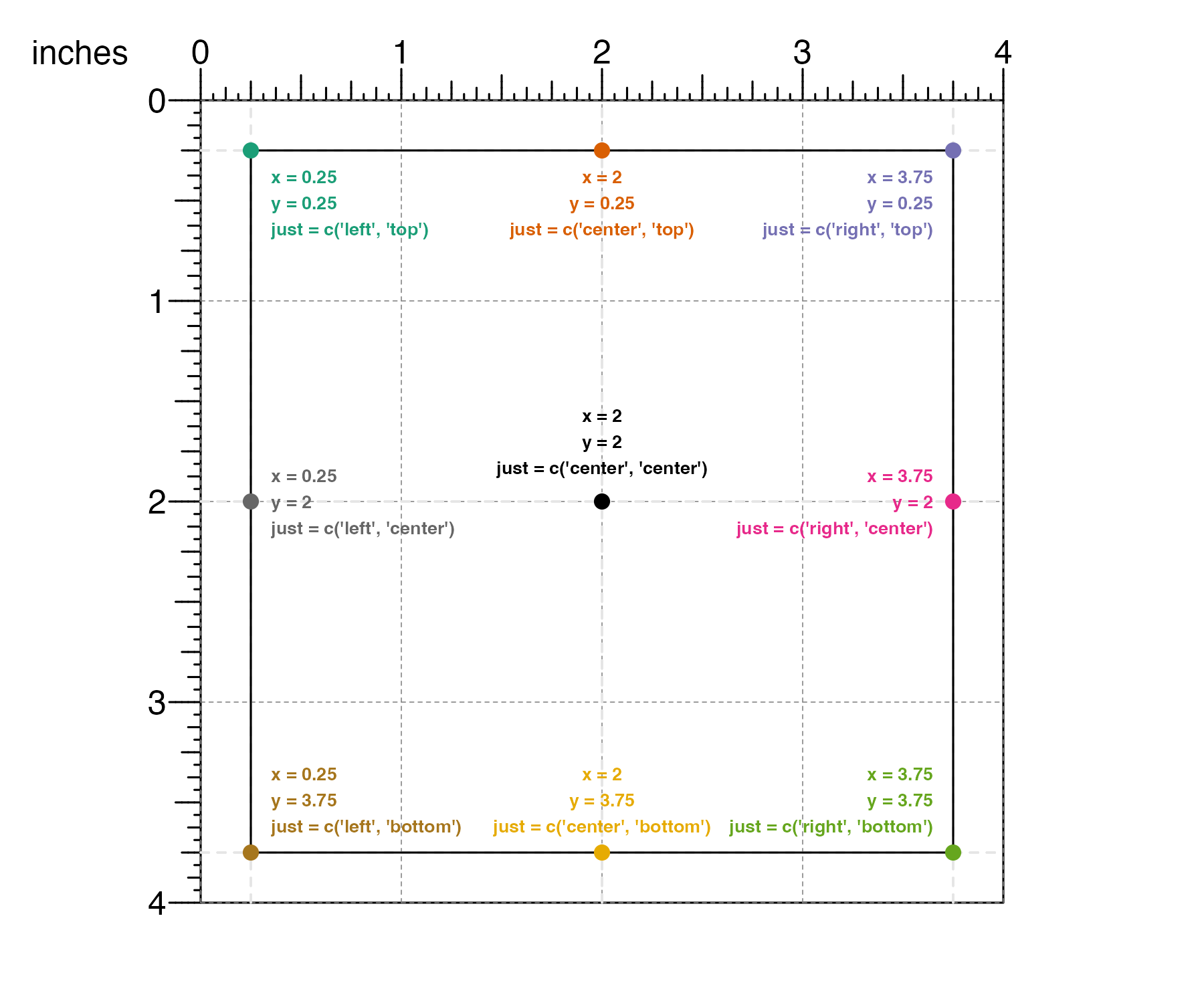
Using the just parameter
While the x, y, width, and
height parameters are relative to the top-left corner of
the plot by default, the just parameter provides additional
flexibility by allowing users to change the placement reference point.
The just parameter accepts a character or numeric vector of
length 2 describing the horizontal and vertical justification (or
reference point), respectively.
The just parameter can be set using character strings
"left", "right", "center",
"bottom" and "top":
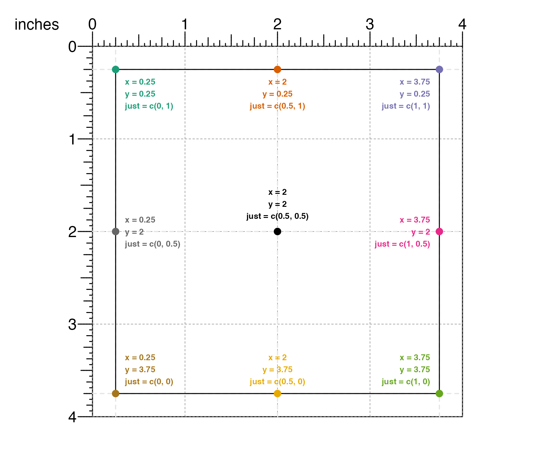
Or it can be set using numeric values where 0 means left/bottom, 1 means right/top, and 0.5 means center:
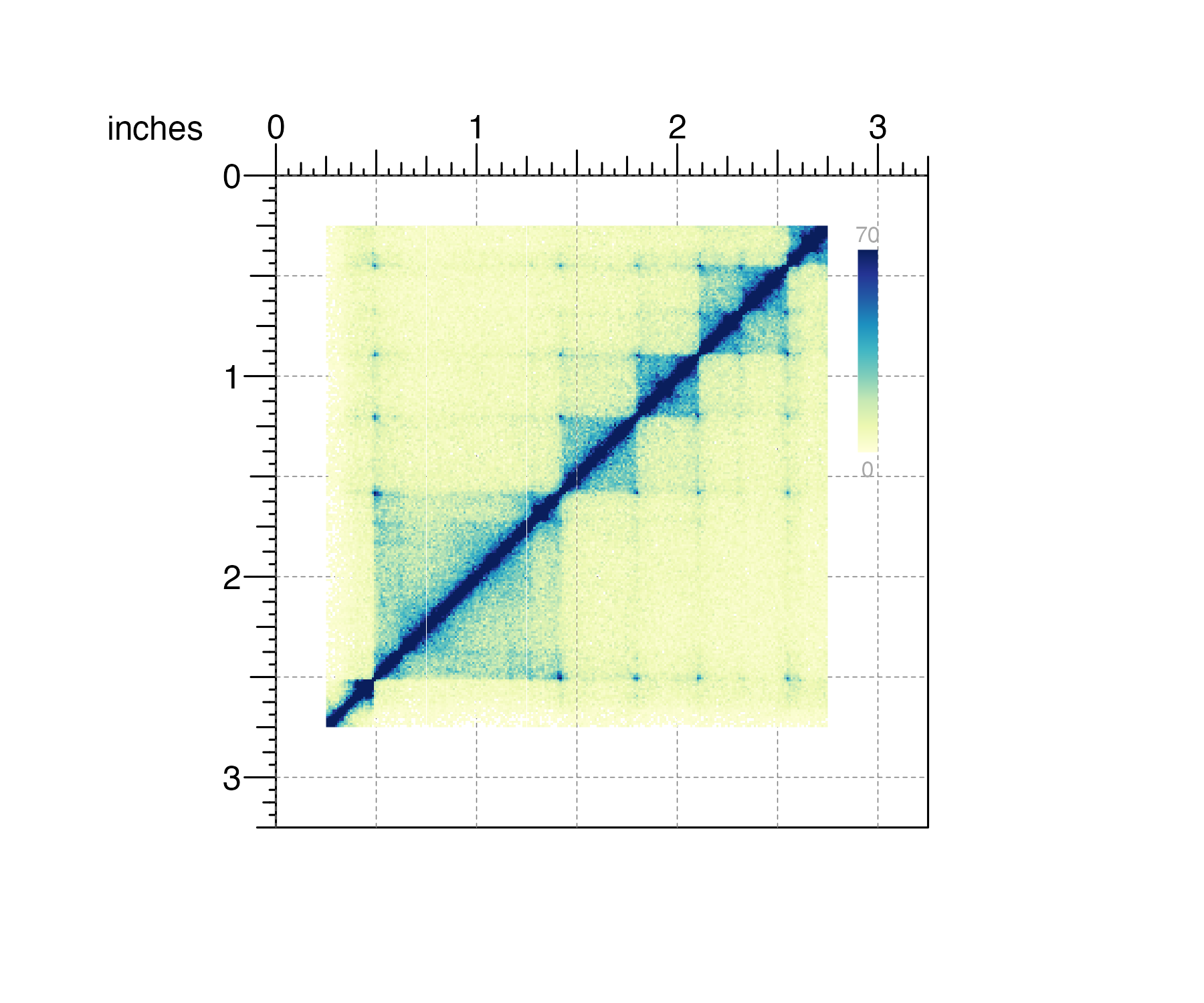
This is particularly useful when an object needs to be aligned in
reference to another plot object or page marker. For example, in the
Hi-C plot below we might want to align the top-right corner of the
heatmap legend to the 3-inch mark. There is no need to calculate the
top-left position (i.e. 3 inches - (legend width)) to
determine where to place the heatmap legend. Instead we can change the
just parameter to just=c('right', 'top'):
## Load example Hi-C data
library(plotgardenerData)
data("IMR90_HiC_10kb")

## Create a plotgardener page
pageCreate(width = 3.25, height = 3.25, default.units = "inches")

## Plot Hi-C data with placing information
hicPlot <- plotHicSquare(
    data = IMR90_HiC_10kb,
    chrom = "chr21", chromstart = 28000000, chromend = 30300000,
    assembly = "hg19",
    x = 0.25, y = 0.25, width = 2.5, height = 2.5, default.units = "inches"
)

## Add color scale annotation with just = c("right", "top")
annoHeatmapLegend(
    plot = hicPlot,
    x = 3, y = 0.25, width = 0.1, height = 1.25,
    just = c("right", "top"), default.units = "inches"
)
Session Info
sessionInfo()
#> R version 4.6.0 (2026-04-24)
#> Platform: aarch64-apple-darwin23
#> Running under: macOS Tahoe 26.5.1
#>
#> Matrix products: default
#> BLAS:   /Library/Frameworks/R.framework/Versions/4.6/Resources/lib/libRblas.0.dylib
#> LAPACK: /Library/Frameworks/R.framework/Versions/4.6/Resources/lib/libRlapack.dylib;  LAPACK version 3.12.1
#>
#> locale:
#> [1] en_US.UTF-8/en_US.UTF-8/en_US.UTF-8/C/en_US.UTF-8/en_US.UTF-8
#>
#> time zone: America/New_York
#> tzcode source: internal
#>
#> attached base packages:
#> [1] grid      stats     graphics  grDevices utils     datasets  methods
#> [8] base
#>
#> other attached packages:
#> [1] plotgardenerData_1.18.0 plotgardener_1.18.0
#>
#> loaded via a namespace (and not attached):
#>  [1] SummarizedExperiment_1.42.0 gtable_0.3.6
#>  [3] rjson_0.2.23                xfun_0.59
#>  [5] bslib_0.11.0                ggplot2_4.0.3
#>  [7] htmlwidgets_1.6.4           plyranges_1.32.0
#>  [9] rhdf5_2.56.0                Biobase_2.72.0
#> [11] lattice_0.22-9              rhdf5filters_1.24.0
#> [13] bitops_1.0-9                vctrs_0.7.3
#> [15] tools_4.6.0                 generics_0.1.4
#> [17] yulab.utils_0.2.4           parallel_4.6.0
#> [19] stats4_4.6.0                curl_7.1.0
#> [21] tibble_3.3.1                pkgconfig_2.0.3
#> [23] Matrix_1.7-5                data.table_1.18.4
#> [25] ggplotify_0.1.3             RColorBrewer_1.1-3
#> [27] cigarillo_1.2.0             S7_0.2.2
#> [29] desc_1.4.3                  S4Vectors_0.50.1
#> [31] lifecycle_1.0.5             compiler_4.6.0
#> [33] farver_2.1.2                Rsamtools_2.28.0
#> [35] textshaping_1.0.5           Biostrings_2.80.1
#> [37] codetools_0.2-20            Seqinfo_1.2.0
#> [39] GenomeInfoDb_1.48.0         htmltools_0.5.9
#> [41] sass_0.4.10                 RCurl_1.98-1.19
#> [43] yaml_2.3.12                 pillar_1.11.1
#> [45] pkgdown_2.2.0               crayon_1.5.3
#> [47] jquerylib_0.1.4             BiocParallel_1.46.0
#> [49] cachem_1.1.0                DelayedArray_0.38.2
#> [51] abind_1.4-8                 tidyselect_1.2.1
#> [53] digest_0.6.39               purrr_1.2.2
#> [55] restfulr_0.0.17             dplyr_1.2.1
#> [57] fastmap_1.2.0               cli_3.6.6
#> [59] SparseArray_1.12.2          magrittr_2.0.5
#> [61] S4Arrays_1.12.0             XML_3.99-0.23
#> [63] withr_3.0.3                 scales_1.4.0
#> [65] UCSC.utils_1.8.0            rappdirs_0.3.4
#> [67] rmarkdown_2.31              XVector_0.52.0
#> [69] httr_1.4.8                  matrixStats_1.5.0
#> [71] otel_0.2.0                  ragg_1.5.2
#> [73] evaluate_1.0.5              knitr_1.51
#> [75] BiocIO_1.22.0               GenomicRanges_1.64.0
#> [77] IRanges_2.46.0              rtracklayer_1.72.0
#> [79] gridGraphics_0.5-1          rlang_1.2.0
#> [81] Rcpp_1.1.1-1.1              glue_1.8.1
#> [83] BiocGenerics_0.58.1         jsonlite_2.0.0
#> [85] strawr_0.0.92               Rhdf5lib_2.0.0
#> [87] R6_2.6.1                    MatrixGenerics_1.24.0
#> [89] GenomicAlignments_1.48.0    systemfonts_1.3.2
#> [91] fs_2.1.0