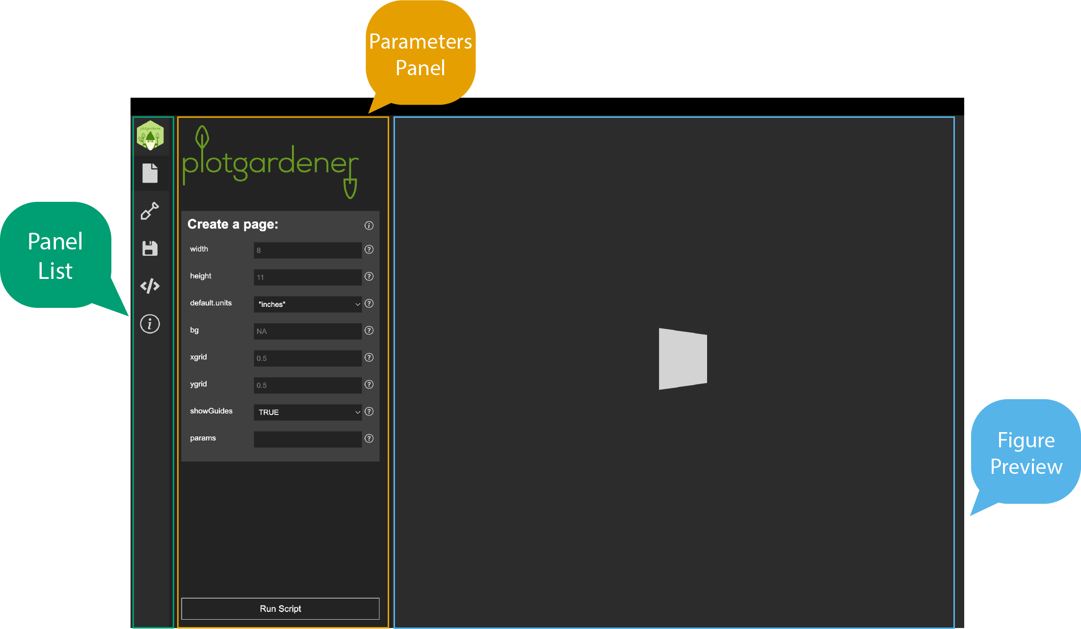
The Plotgardener App interface is divided into three regions: the Panel List, the Parameters Panel, and the Figure Preview. The Panel List on the left provides icon-based navigation between four sections — Page, Plots, Save, and Code. The Parameters Panel in the center displays the relevant controls for whichever section is active. The Figure Preview on the right shows a live rendering of your figure. This guide walks through each section and describes a typical workflow for building a figure from start to finish.

The Page Tab
Before adding any plots, use the Page tab to set the overall canvas dimensions for your figure. Its settings appear in the Parameters Panel.
Settings available:
- Width / Height: Physical dimensions of the output figure (in the selected units).
-
Units: Choose from inches (
in), centimeters (cm), or millimeters (mm). - Default parameters: Set package-wide defaults — such as genome assembly or font size — that apply across all panels unless overridden at the panel level.
Once you have configured the page, click Run Script to render a blank page in the Figure Preview. Page dimensions directly determine the size of the exported PDF. If you are targeting a specific journal figure size (e.g., single-column = 3.5 in, double-column = 7 in), set those here.
For more on how the plotgardener coordinate system
works, see The plotgardener
Page.

The Plots Tab
The Plots tab is where you add, configure, and arrange individual visualization panels. Select it from the Panel List to load its controls into the Parameters Panel.
Adding a Plot
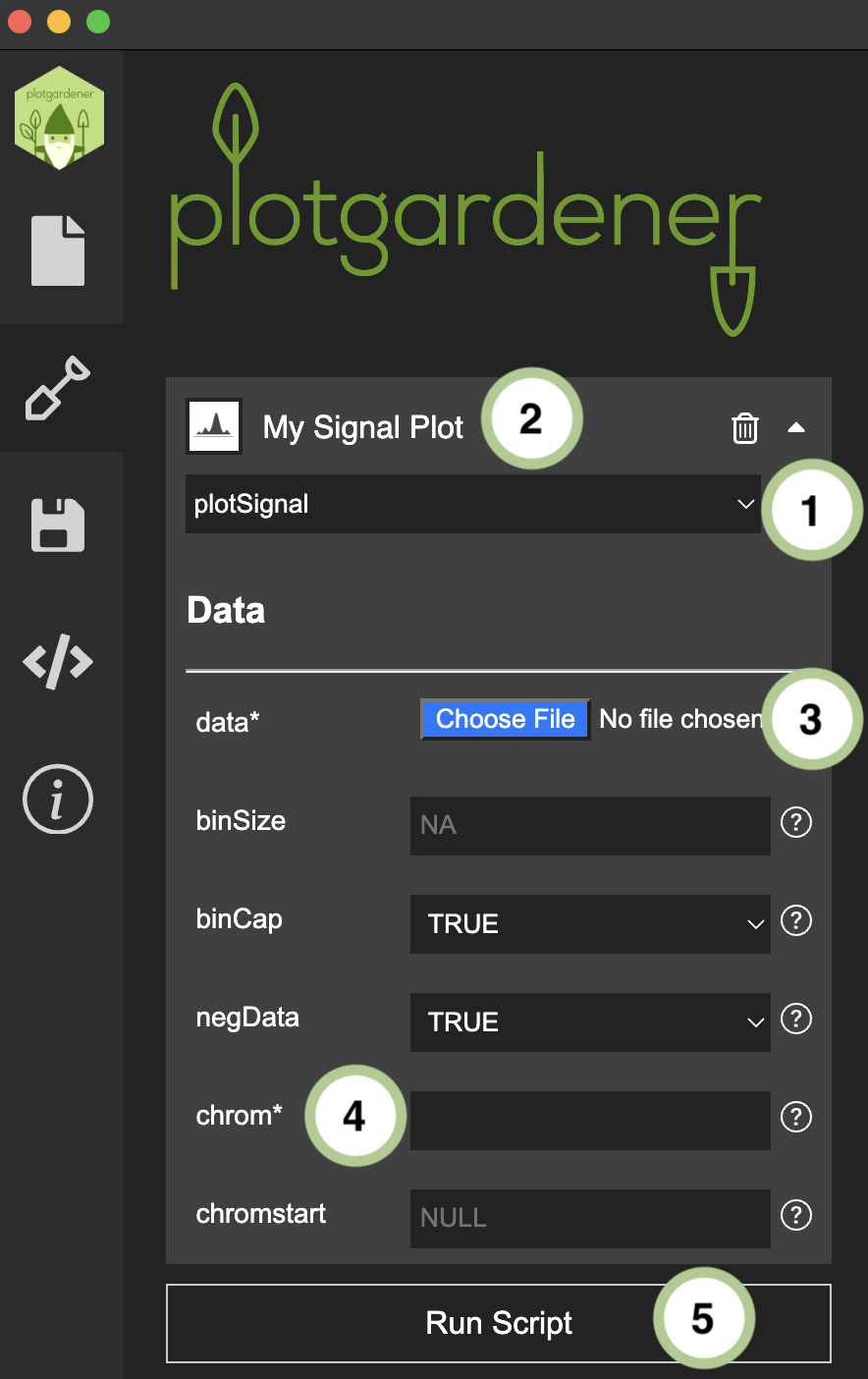
- Select a
plotgardenerfunction from the Function dropdown in the Parameters Panel. All functions supported by the installed version ofplotgardenerare listed automatically. - Give the panel a descriptive name in the Panel Name field.
- Upload your data file using the Browse button next to the relevant data parameter.
- Fill in the required parameters (denoted by
*in the interface). Optional parameters can be left at their defaults. - Click Run Script to render the updated figure in the Figure Preview.
For more information on each type of plot and their input requirements, see Plot Types
Editing a Plot
- Select any existing panel from the Plot List
- Adjust its parameters in the Parameters Panel
- Click Run Script to re-render.
Adding Annotations
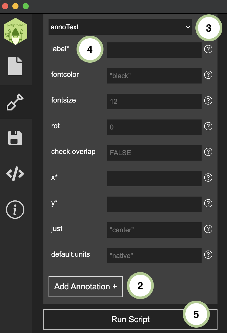
To layer annotations onto an existing plot (e.g., a highlight box, genome axis, or domain boundary):
- Select the target plot from the Plot List, in the Parameters Panel.
- Click the Add Annotation + button at the bottom of the plot’s parameters.
- Choose an annotation function from the Annotations dropdown.
- Configure its parameters.
- Click the Run Script button.
See Plot Types and Annotations for details on available annotation types.

The Save Tab
The Save tab lets you preserve and restore your entire figure session. Select it from the Panel List to access its controls in the Parameters Panel.
-
Save Session: Exports the current configuration —
all panels, parameter values, and page settings — as a structured
.jsonfile. -
Load Session: Imports a previously saved
.jsonfile to restore a figure exactly as it was, including all panels and their parameter values.
Sessions are portable across machines, making it straightforward to share figure templates with collaborators or reproduce figures in a different environment.

The Code Tab
The Code tab displays the R script that the app generates from your current panel configuration. Select it from the Panel List to view the script in the Parameters Panel.
- The script updates in real time as you add, remove, or modify panels.
- Click Copy to copy the full script to your clipboard and paste it into RStudio or any other IDE.
- Advanced users can use this script as a starting point for customization beyond what the GUI supports — adding custom color palettes, looping over multiple regions, or integrating with other Bioconductor objects.
This tab is particularly useful for learning: configure a plot in the
Plots tab, then switch to Code to
inspect the equivalent plotgardener R function calls.
Typical Workflow
A complete figure-building session follows this sequence:
- Set the page — Select the Page tab from the Panel List, enter your figure dimensions and units in the Parameters Panel, and click Run Script.
- Add your first panel — Select the Plots tab, choose a function, upload your data, and enter the genomic coordinates (chromosome, start, end) and any required parameters.
- Preview the figure — Click Run Script. The Figure Preview on the right renders the current figure.
- Add more panels — Repeat steps 2–3 for each additional track or panel, positioning them on the page using the x, y, width, and height parameters.
- Add annotations — Layer genome axis labels, highlight regions, domain boundaries, or other annotations onto existing panels.
-
Save your session — Select the
Save tab and export the session as a
.jsonfile for later use or sharing. - Export the R script — Select the Code tab and copy the generated script for archiving, further customization, or reproducibility.
Further Resources
- Plot Types and Annotations — descriptions and examples of available plotting and annotation functions
- The plotgardener Page — coordinate system and page layout
plotgardenerR package documentation