Plotgardener App Tutorial
Source:vignettes/guides/plotgardenerApp_tutorial.Rmd
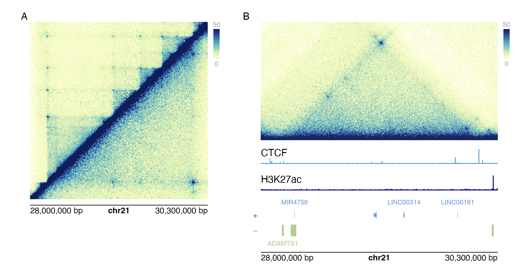
plotgardenerApp_tutorial.RmdLet’s recreate this figure using the Plotgardener App!
Download Sample Data
To plot this figure you will need to download the HiC and bigWig data. To download the data click the links below. These files were created to practice with the tutorial and only contain data for chromosome 21 (and thus are very small files). If you’re interested in plotting other regions in different chromosomes you can provide your own data or download larger publicly available datasets to plot!
(right-click and select “Save link as…” to download)
Getting Started
First, open the Plotgardener App. It should be installed and available as an application on your computer. For installation help, see the installation guide.
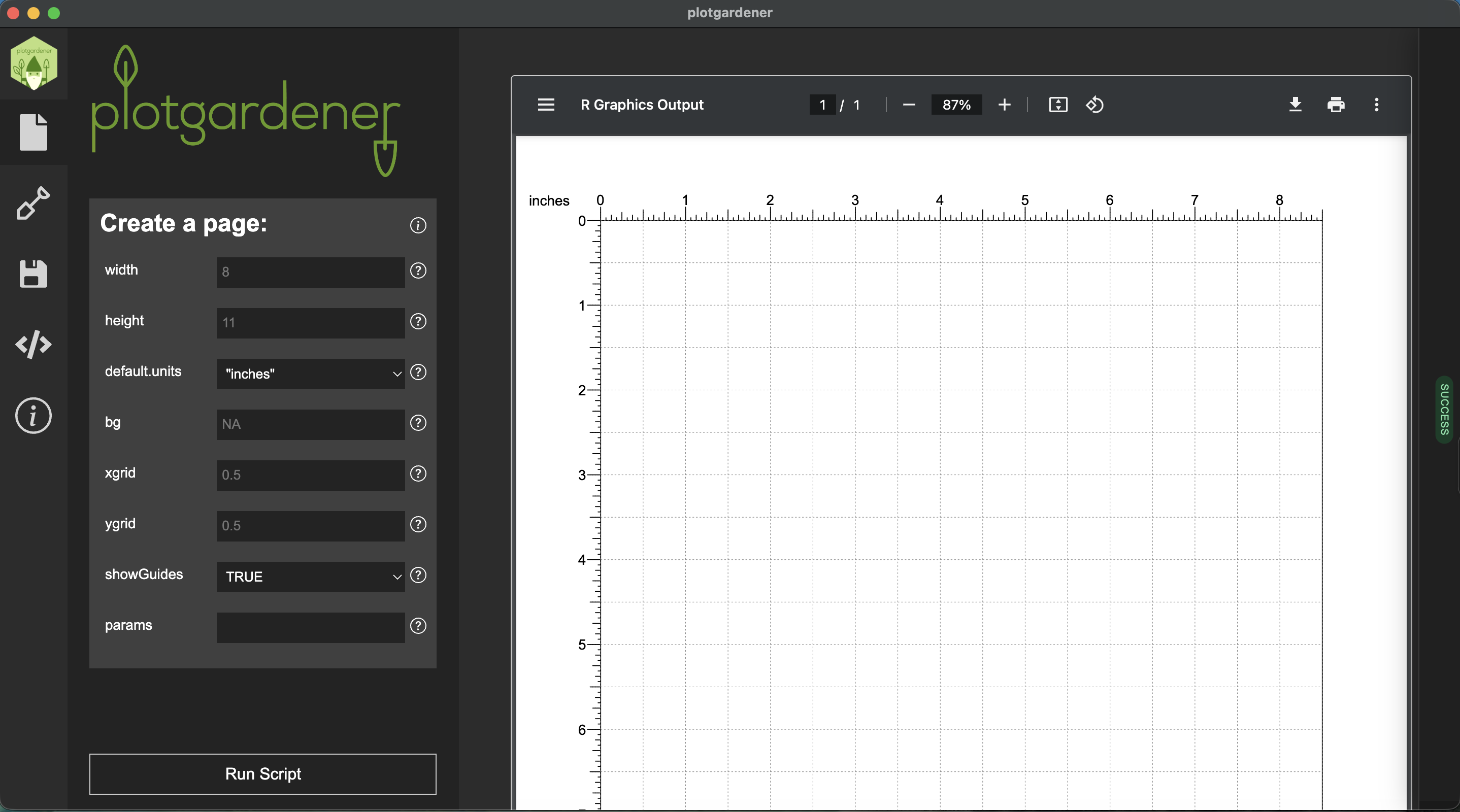
After opening the app, you will see the default page. For an overview of all the tabs, see the User Interface guide.
Create a Custom Page
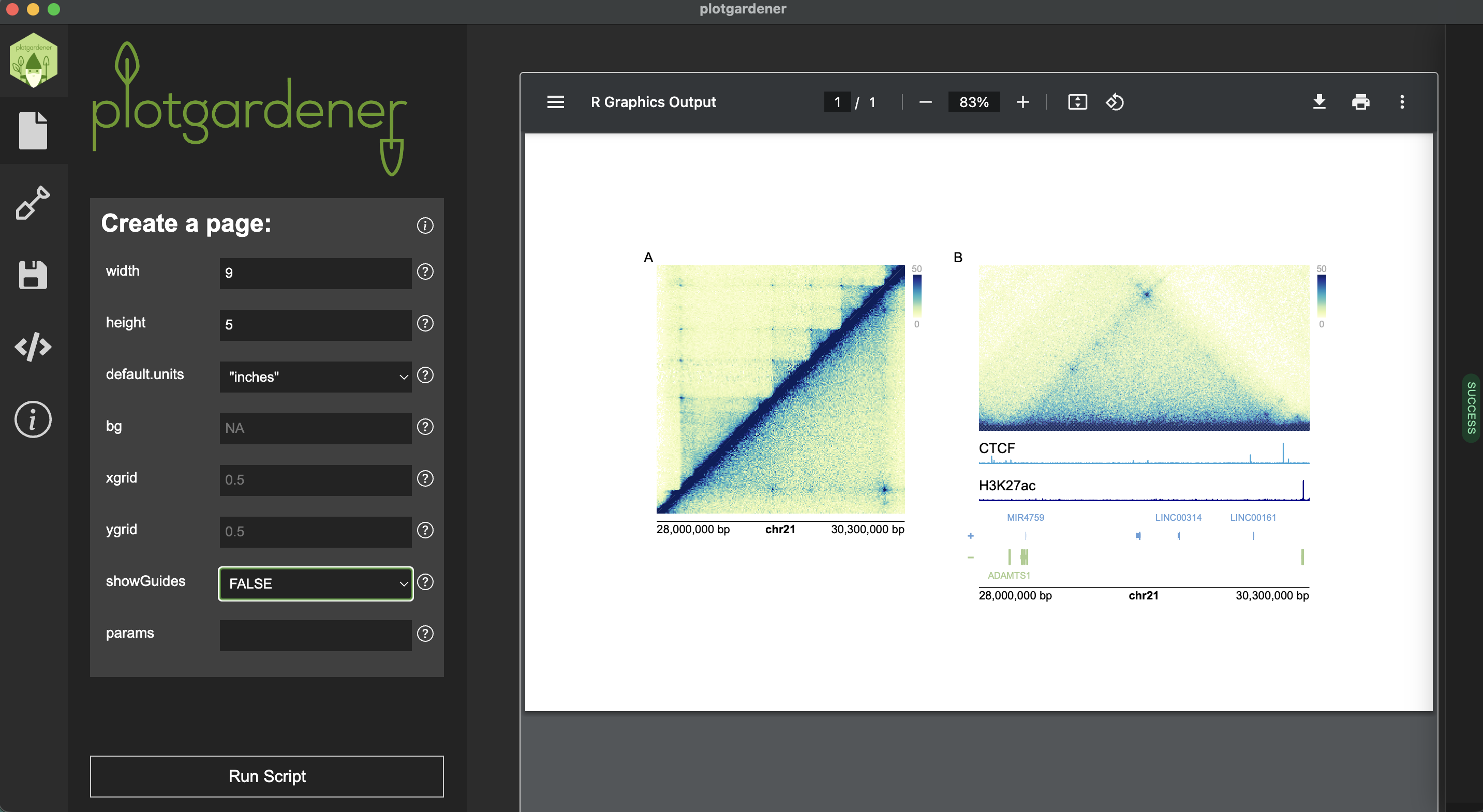
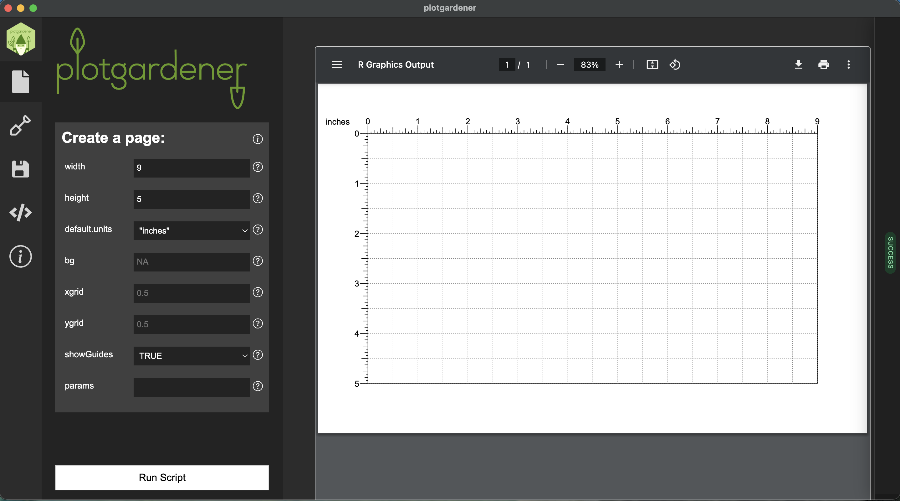
We will start by creating a custom-sized page. Leave Show
Guides set to TRUE so we can map out where we want
our plots.
Set the following values and click Run Script:
Add Panel A — HiC Square Plot (Top Half)
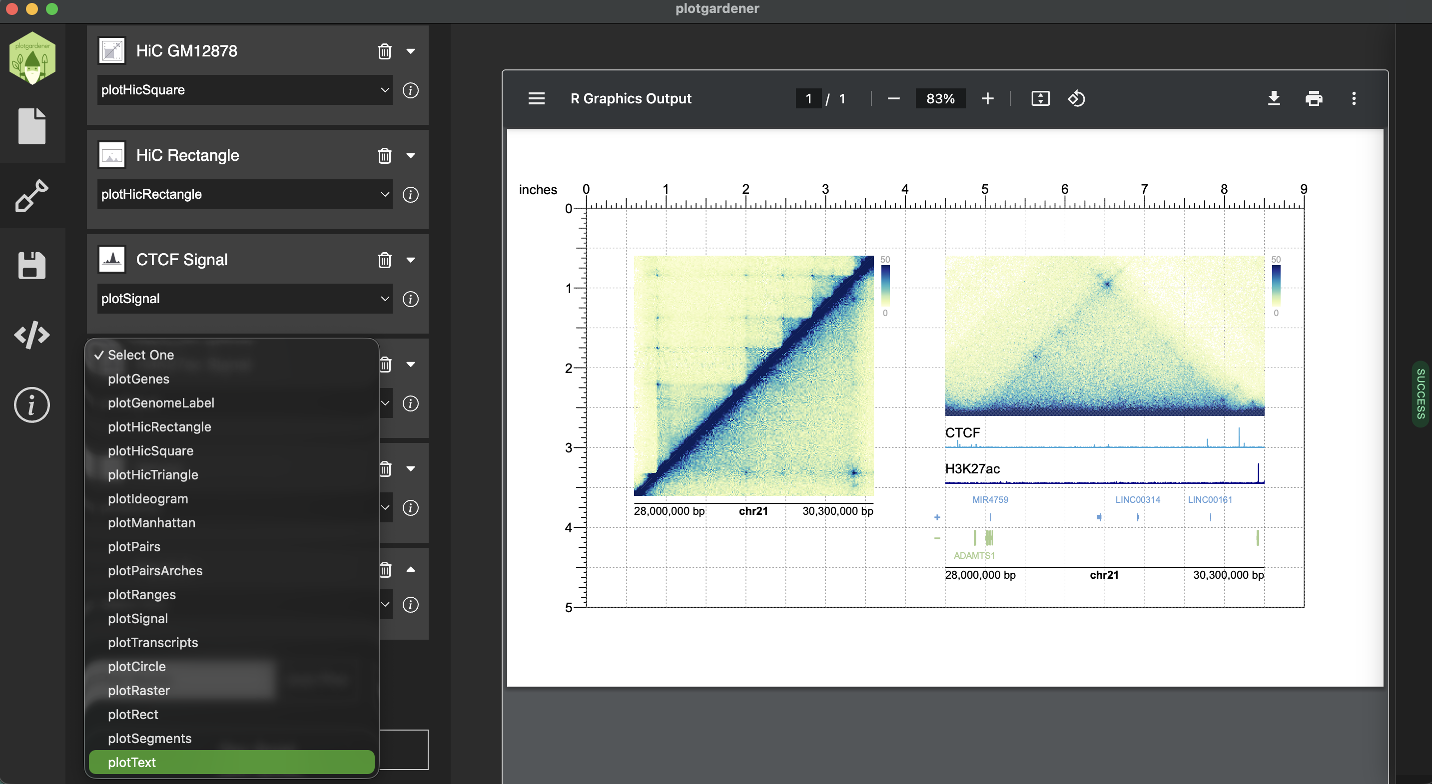
Navigate to the Plots tab (shovel icon) to begin adding plots to the figure.
Add the plot
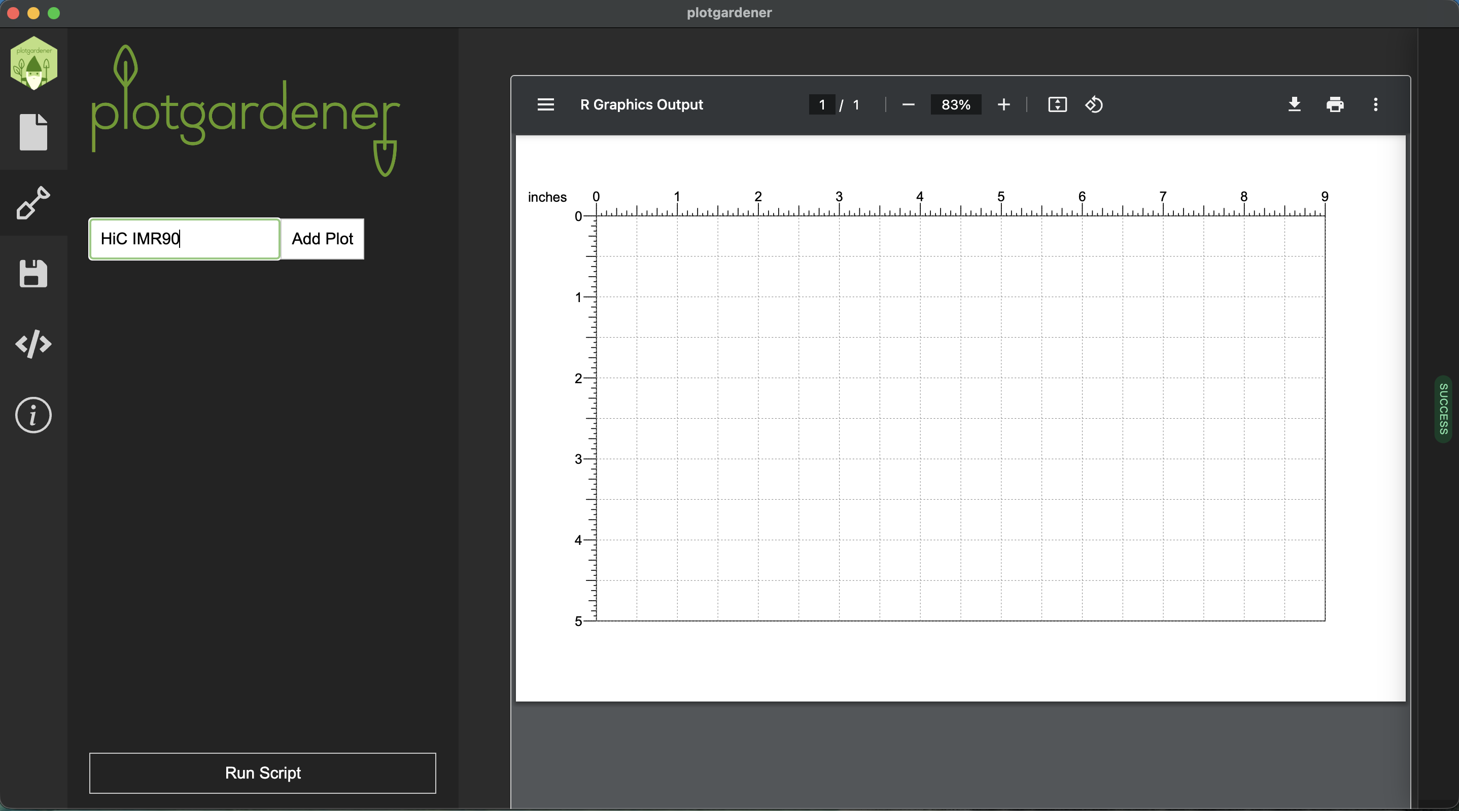
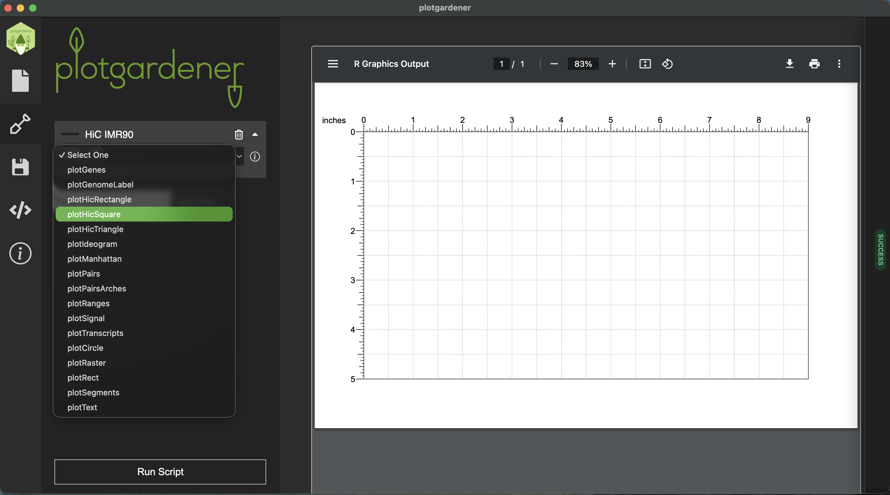
Click Add Plot and give your plot a name, here we’ve named the plot after the file. Select plotHicSquare as the plot type. For an overview of all plot types and their required inputs, see the Plot Types and Annotations guide.
Data parameters
Select the IMR90 HiC file as the input data. Then enter the following data parameters:
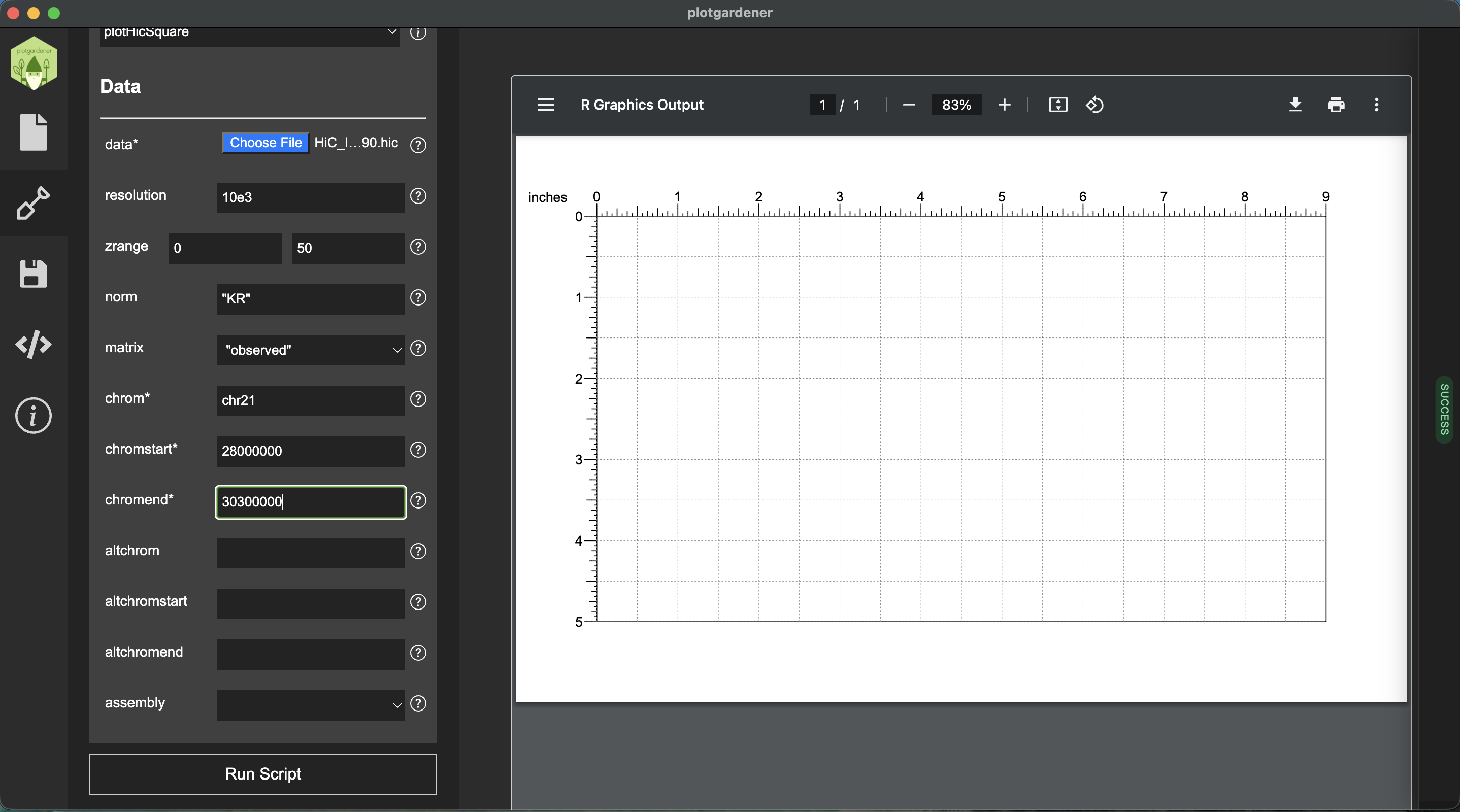
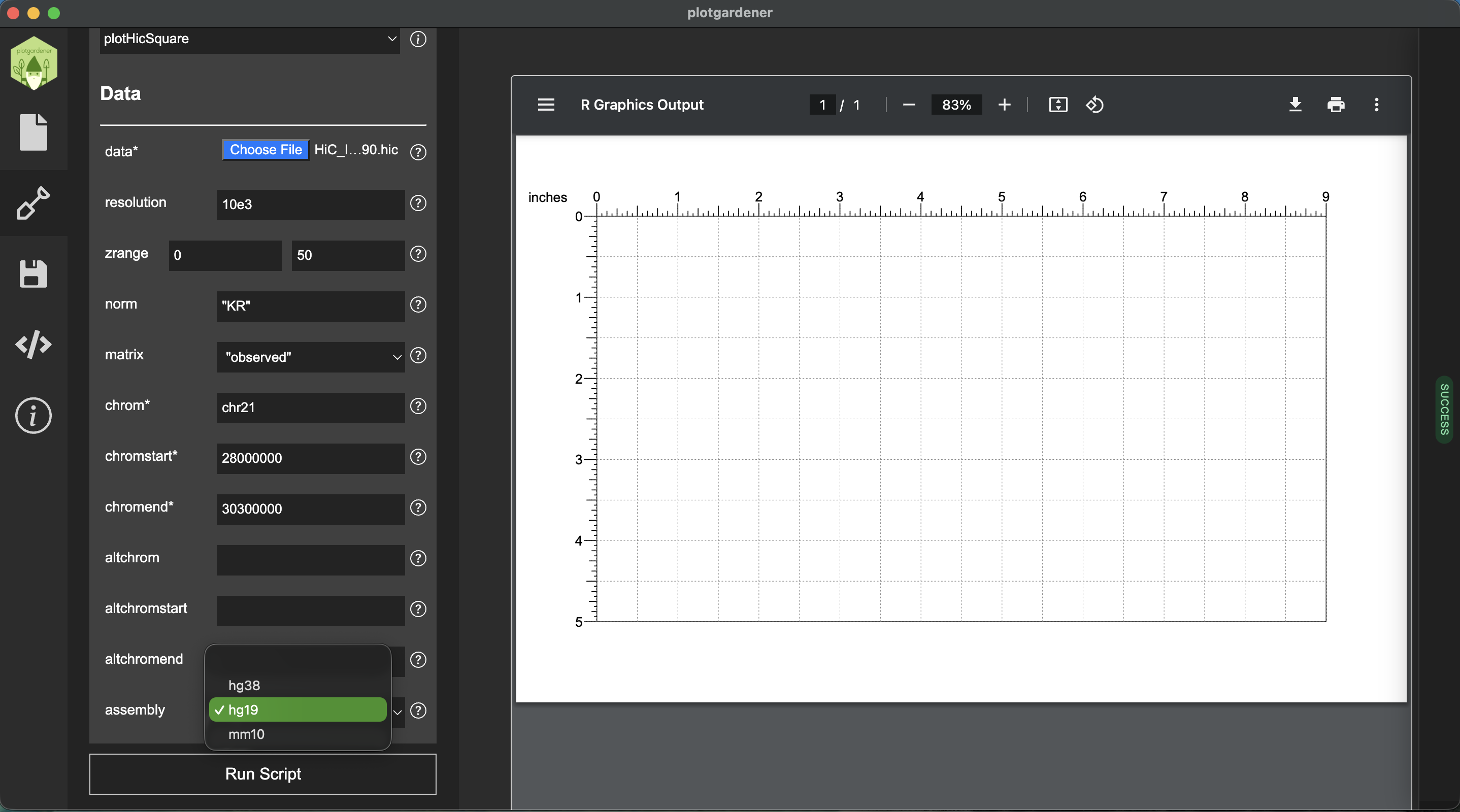
Set the Assembly to hg19, which
indicated which build of the genome our data was aligned to.
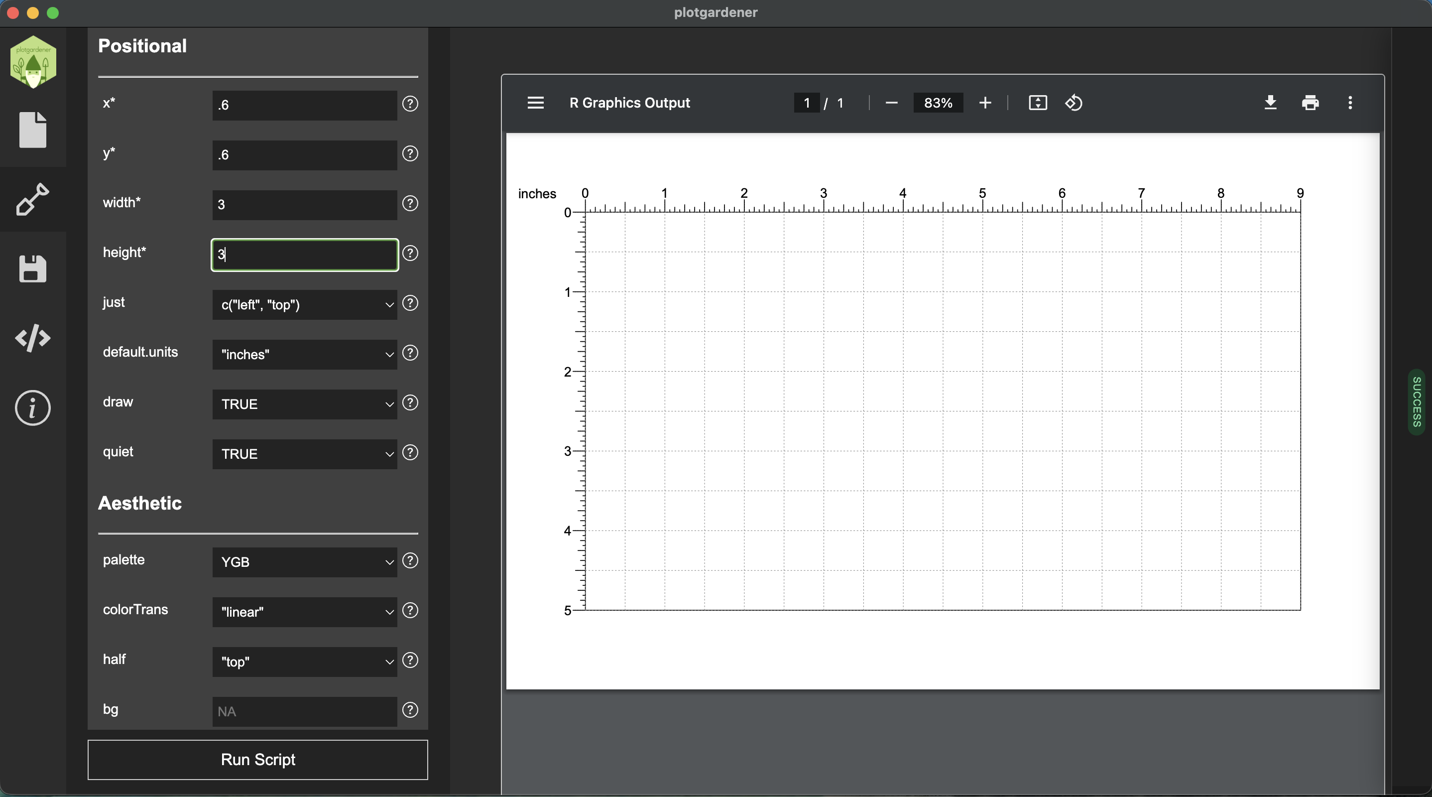
Half
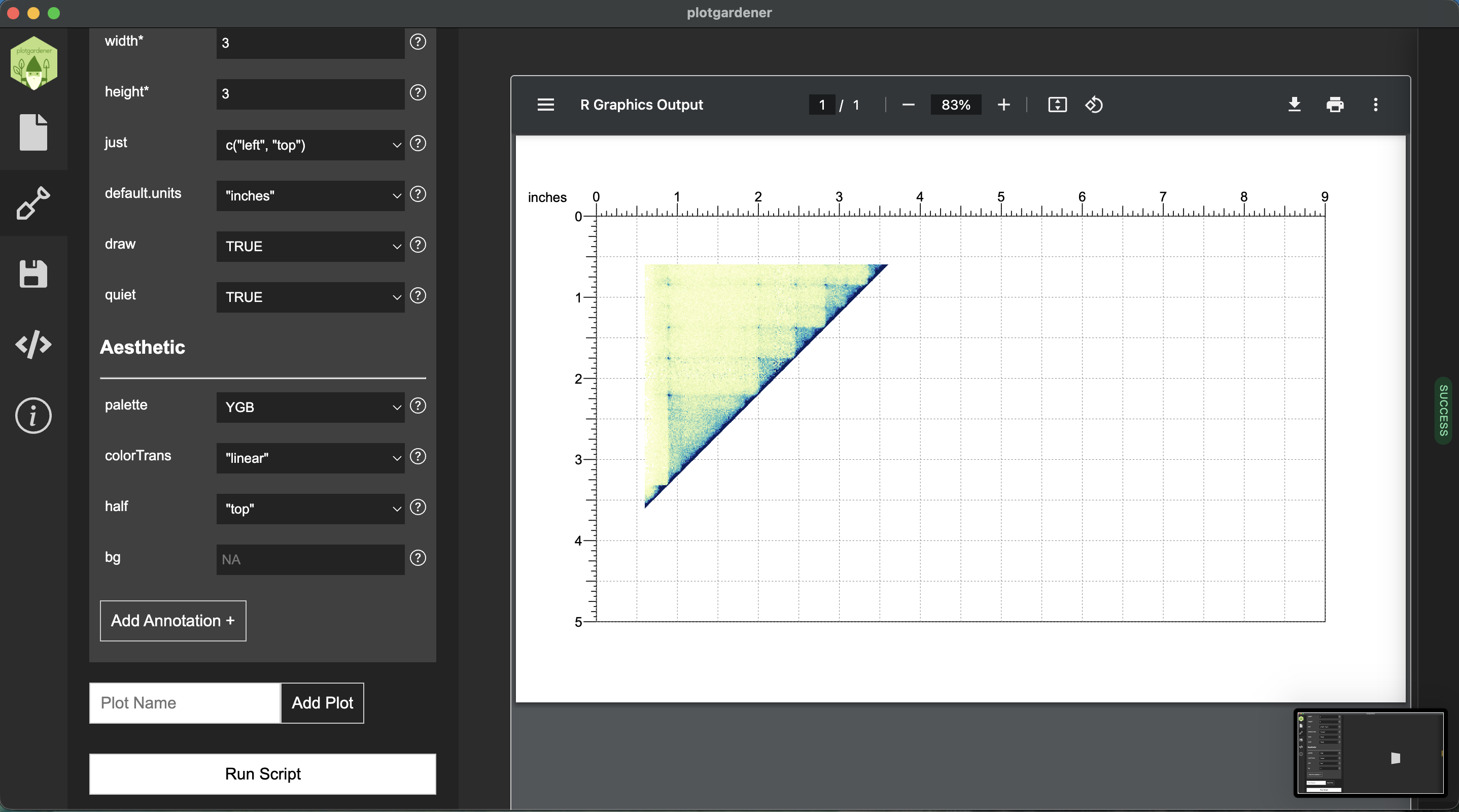
Since we are plotting only the top half of the square, set
Half to top.
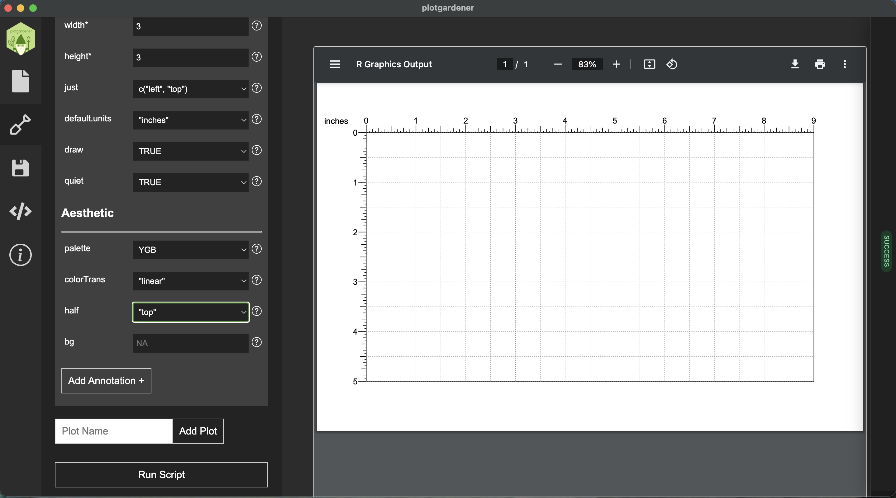
Click Run Script to render the plot.
Annotations
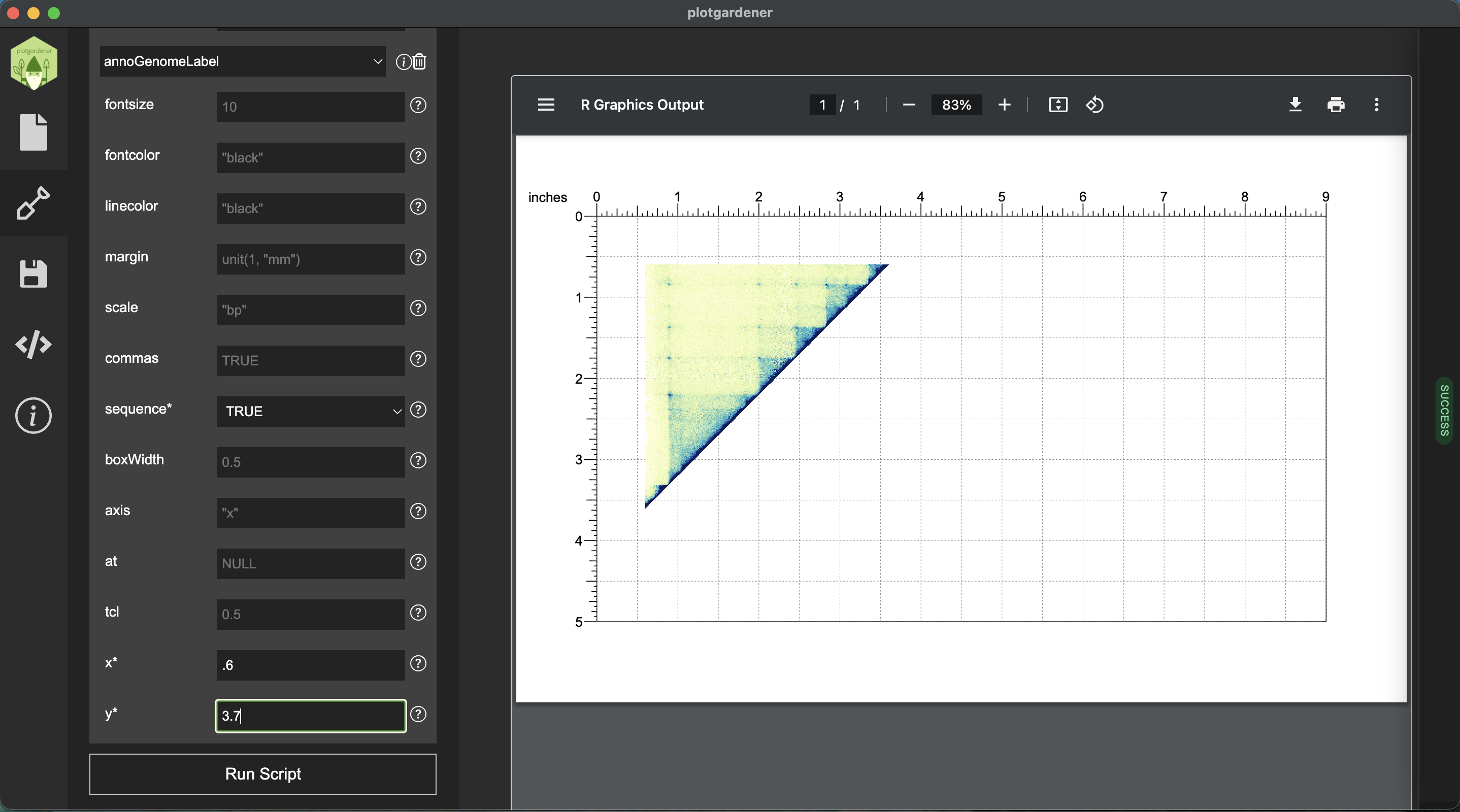
Genome label: Click Add Annotation at the bottom of the HicSquare plot and select annoGenomeLabel. Enter the x and y positions for the label.
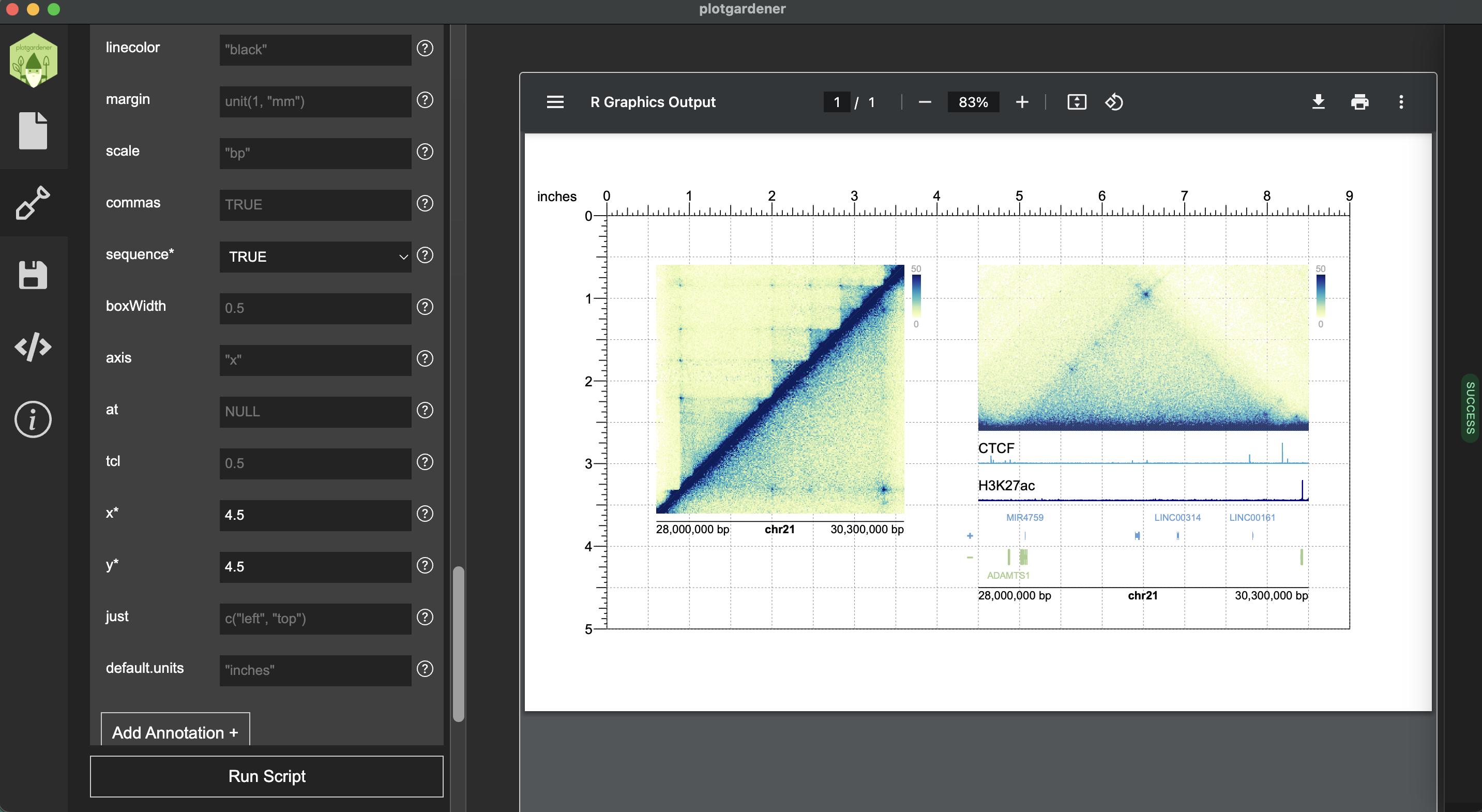
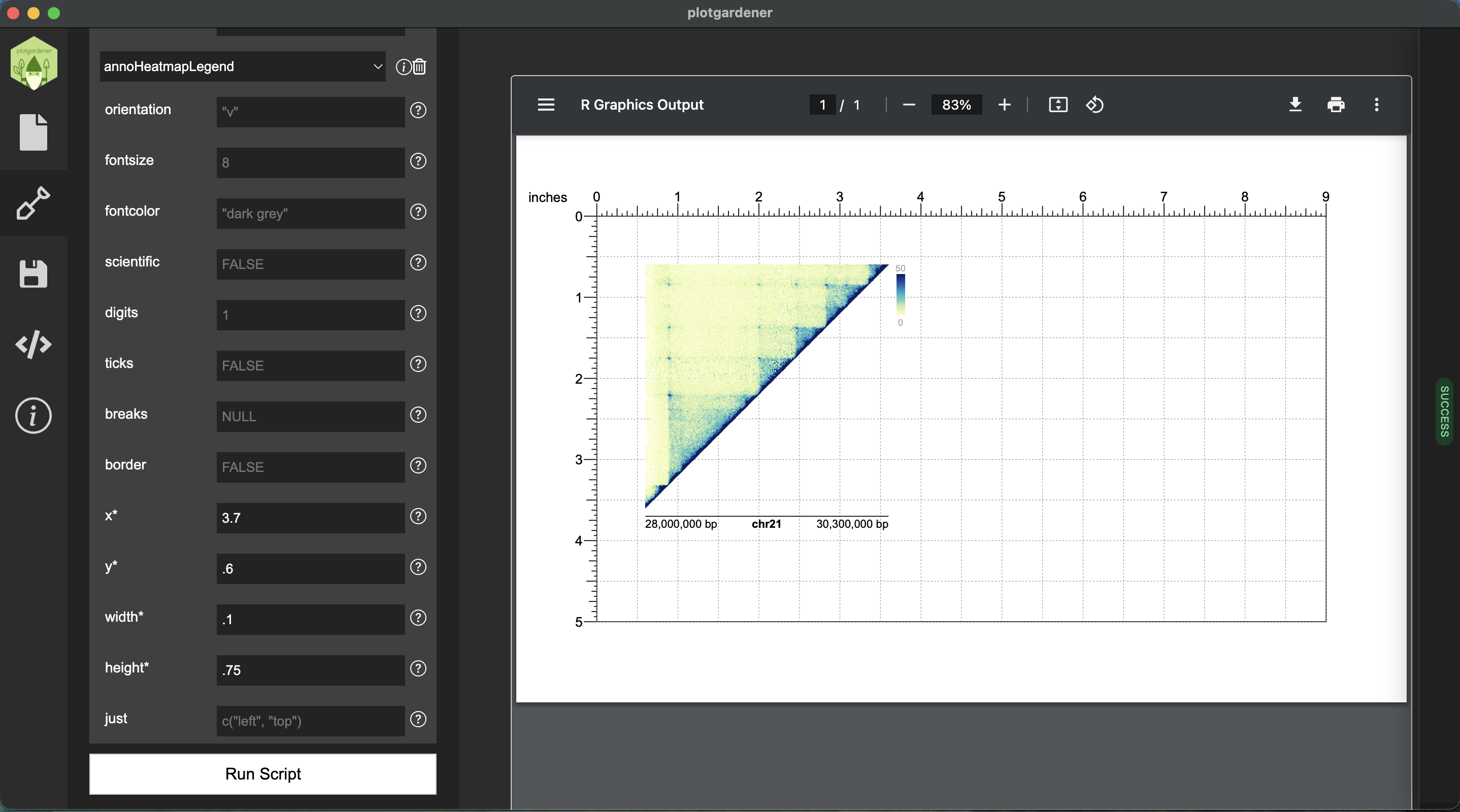
Heatmap scale bar: Click Add Annotation again and select annoHeatmapLegend. Enter the following position and size values:
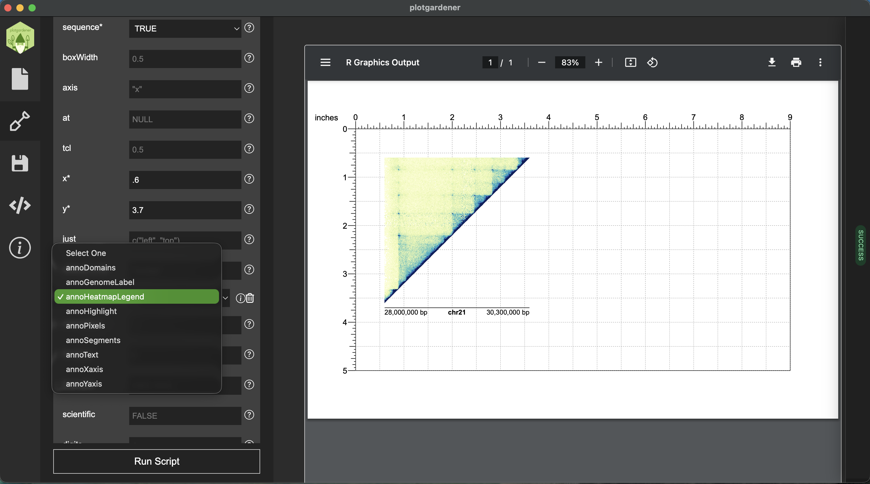
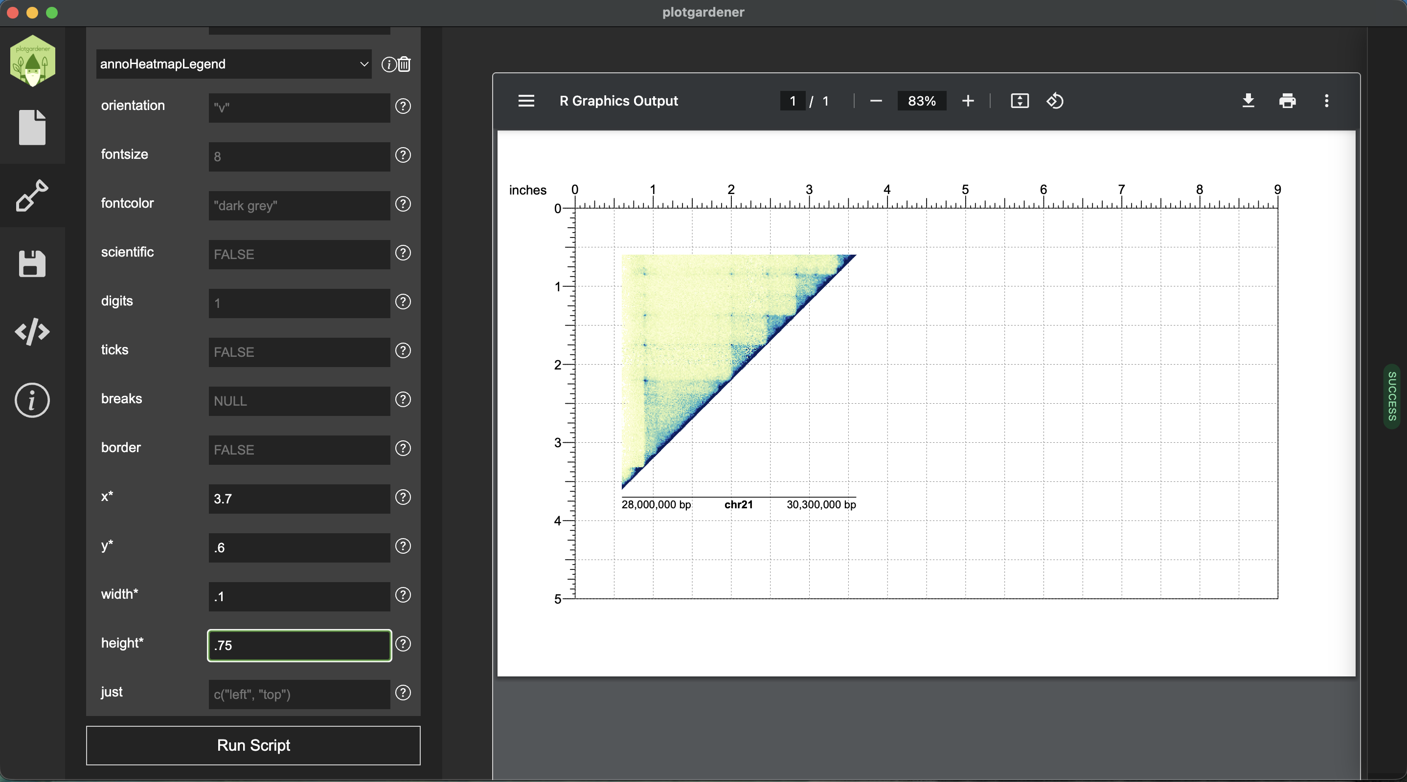
Click Run Script to see the annotations added.
Add Panel A — HiC Square Plot (Bottom Half)
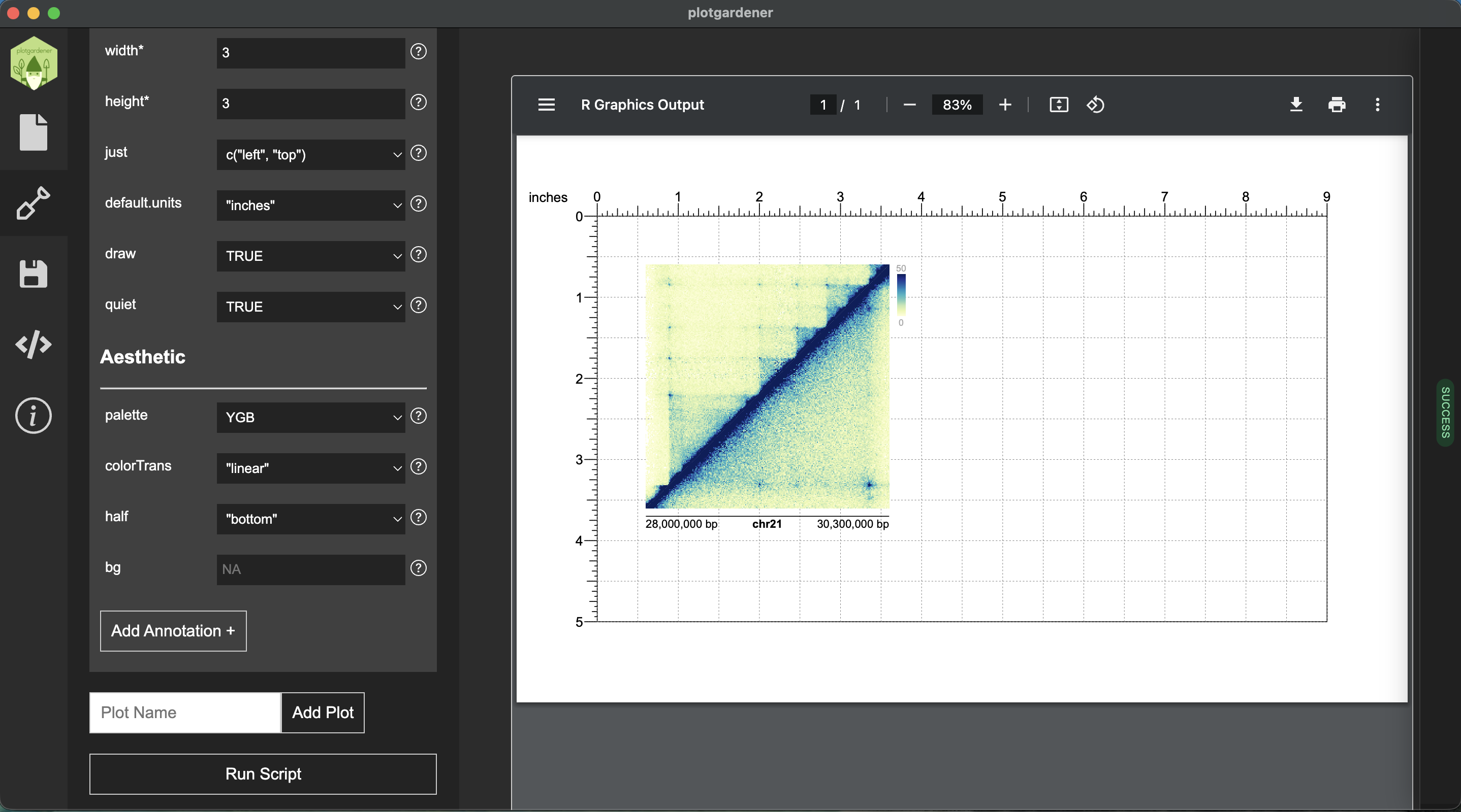
Click Add Plot and add another
plotHicSquare. This time, select the GM12878 HiC file
as the input data file. Enter the same data parameters as before, but
set Half to bottom.
Click Run Script to render the bottom half of the square.
Add Panel B — HiC Rectangle
Click Add Plot and select plotHicRectangle. Choose the GM12878 HiC file as the input data. Enter the same data parameters as before, then add the positional parameters below:
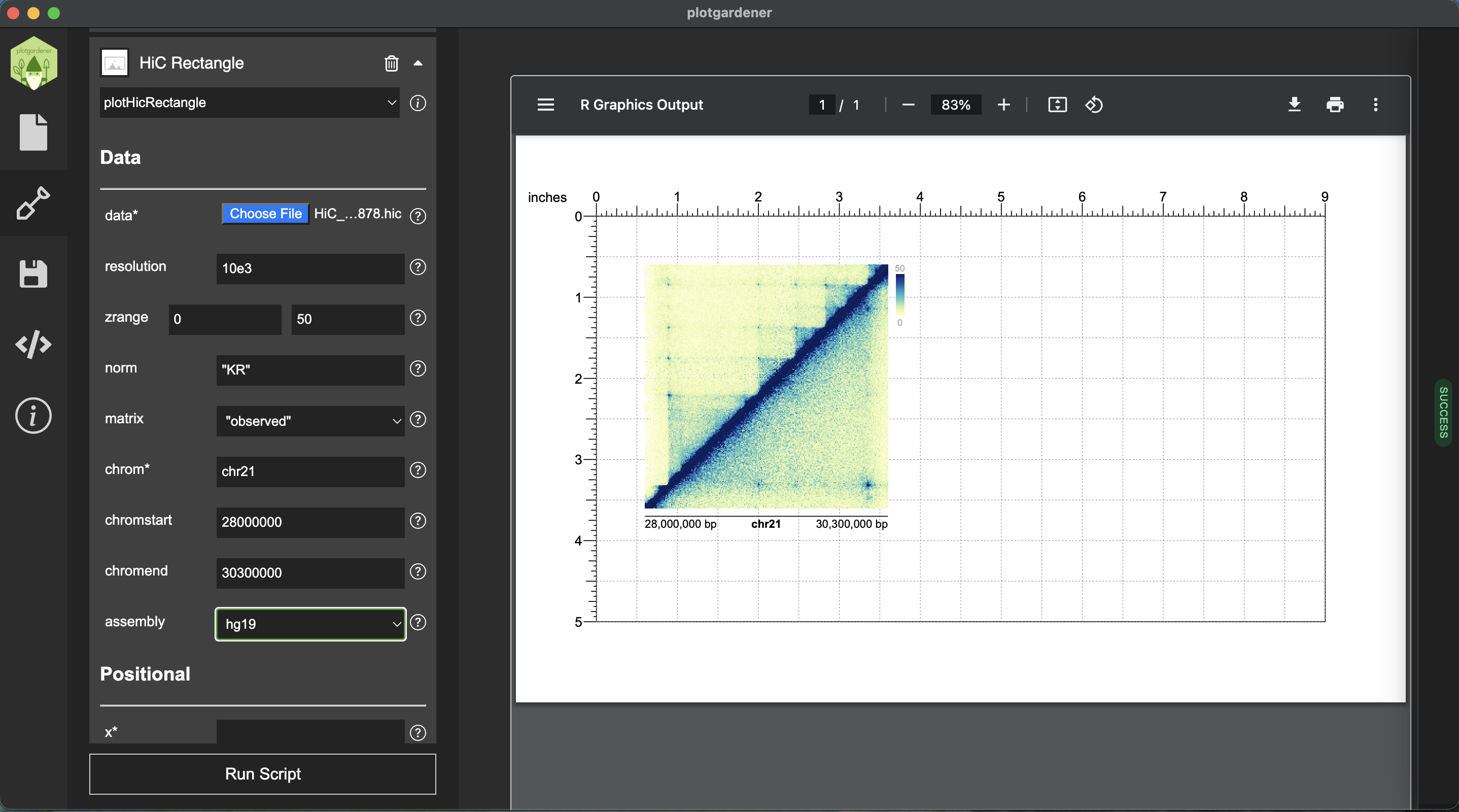
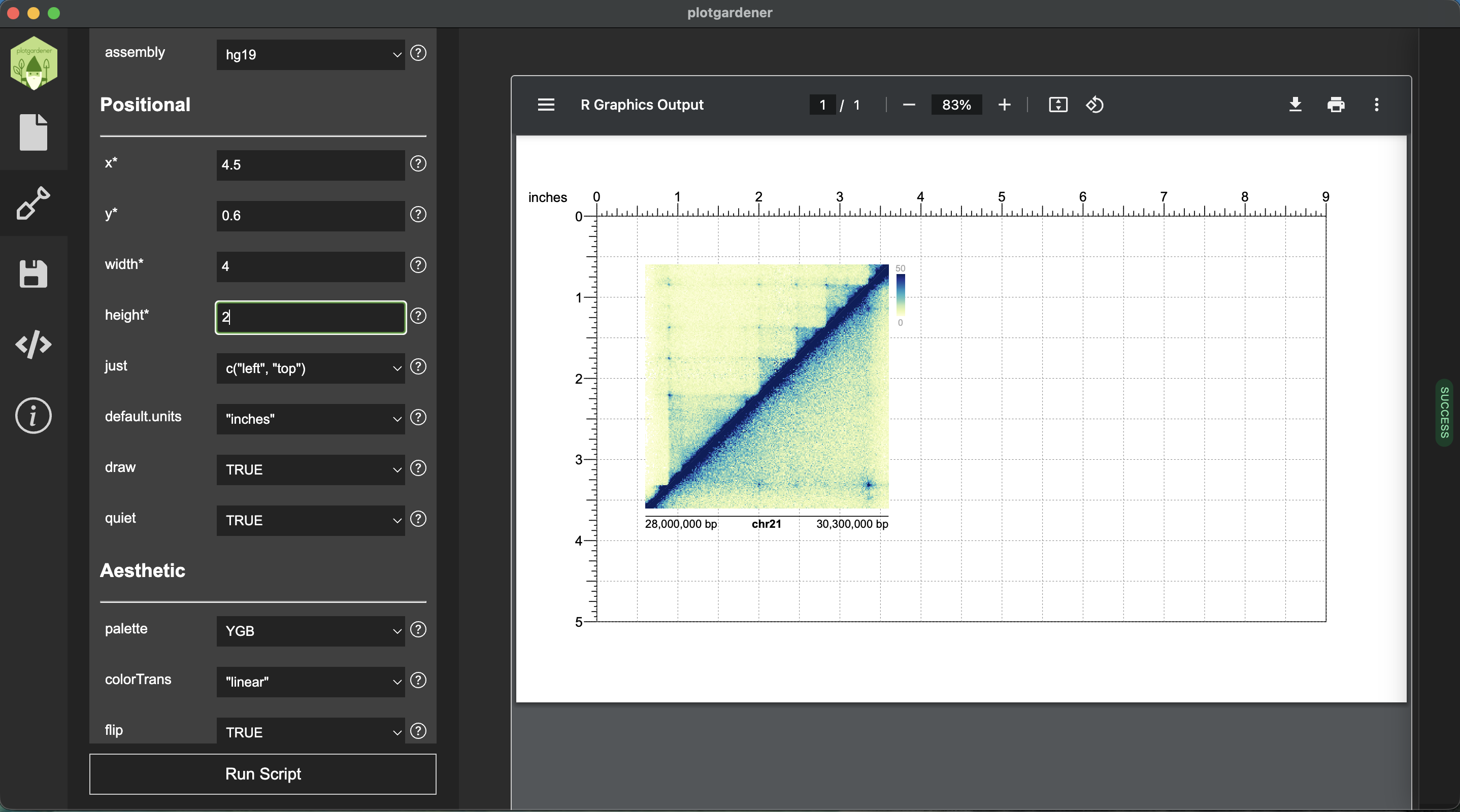
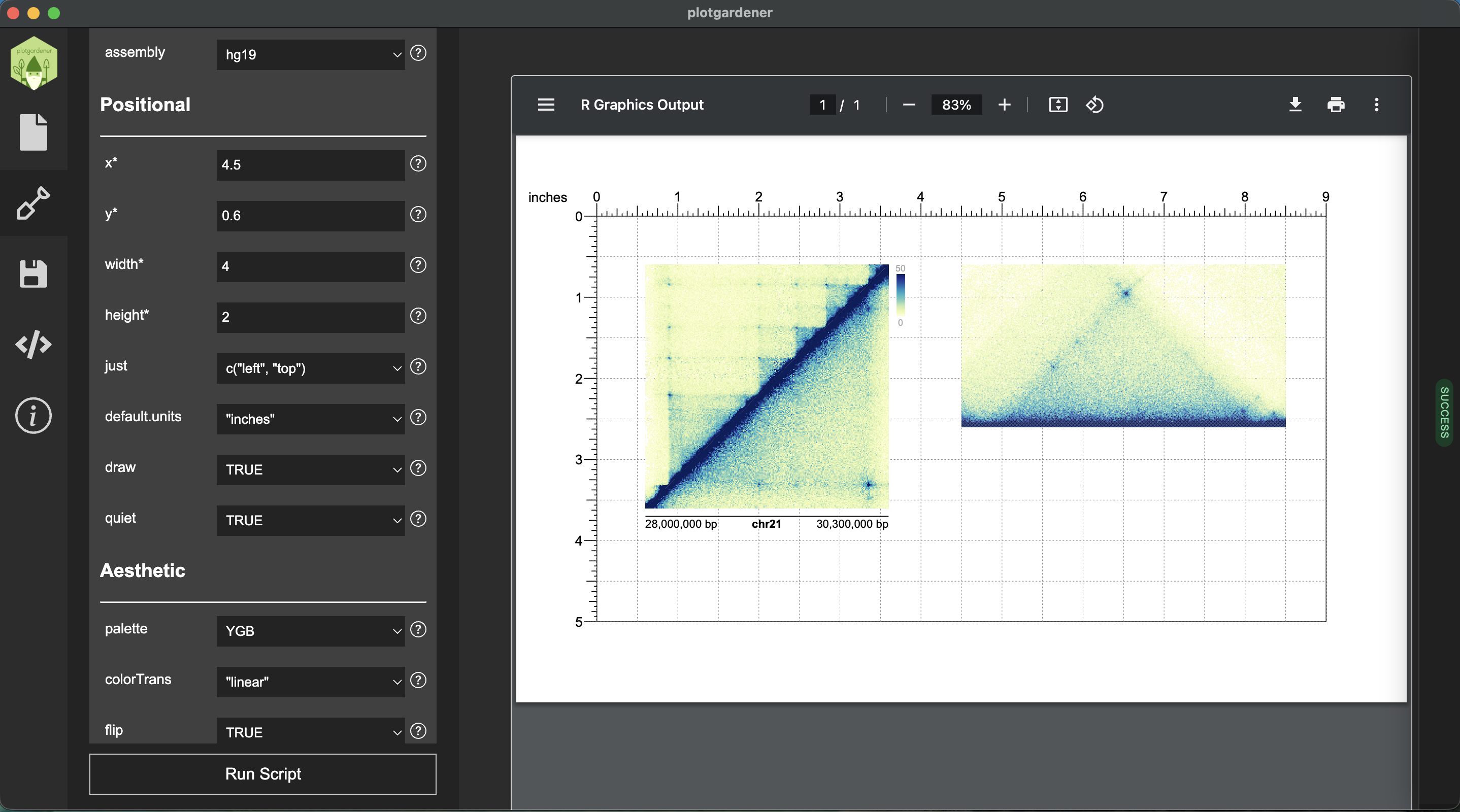
Click Run Script.
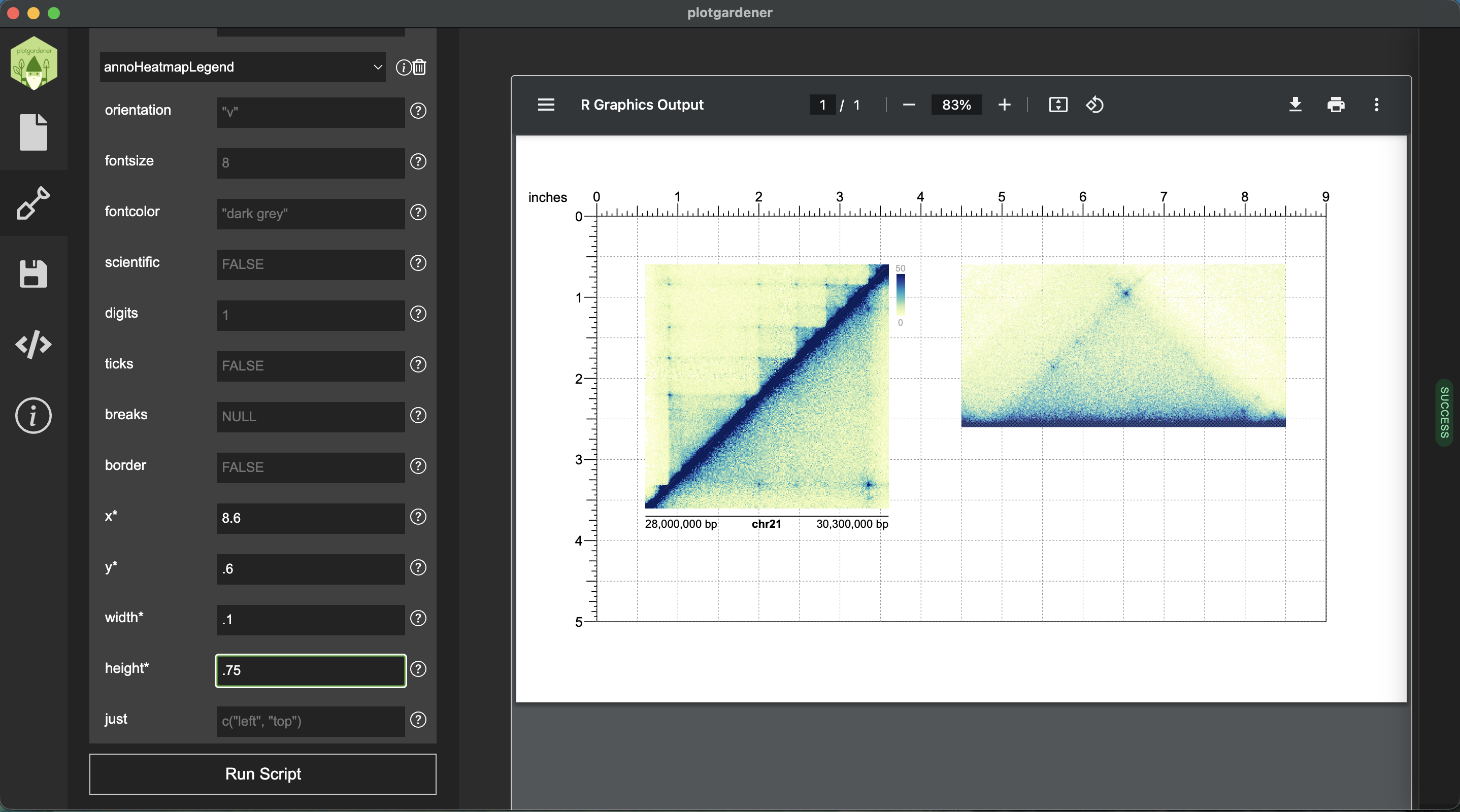
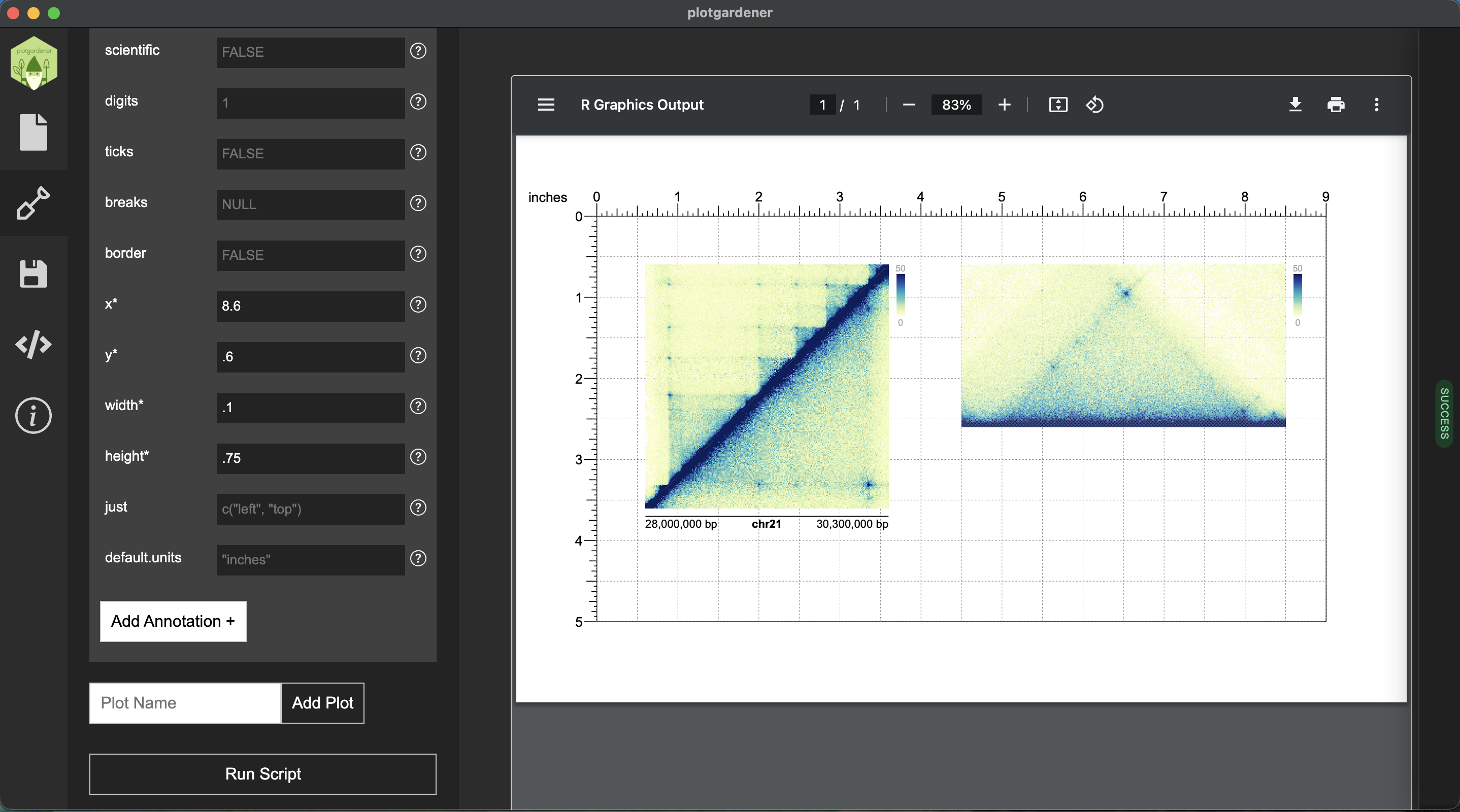
We can also add a scale bar annotation like before.
Add Signal Tracks
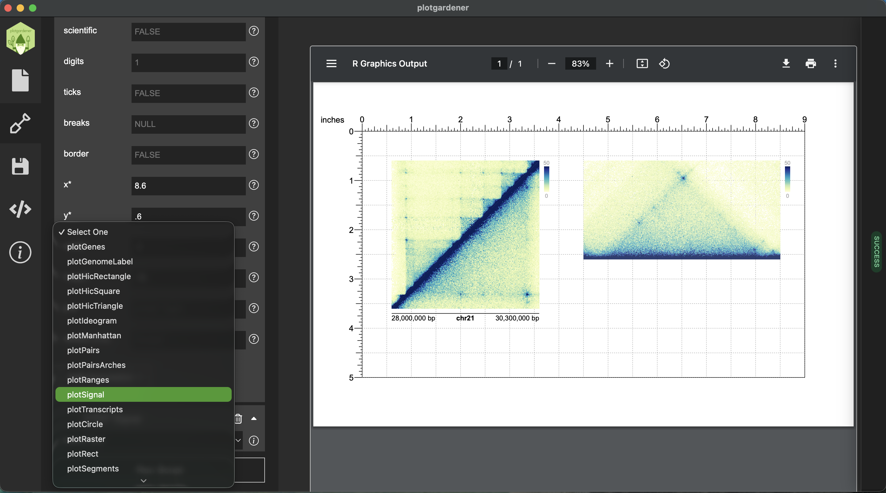
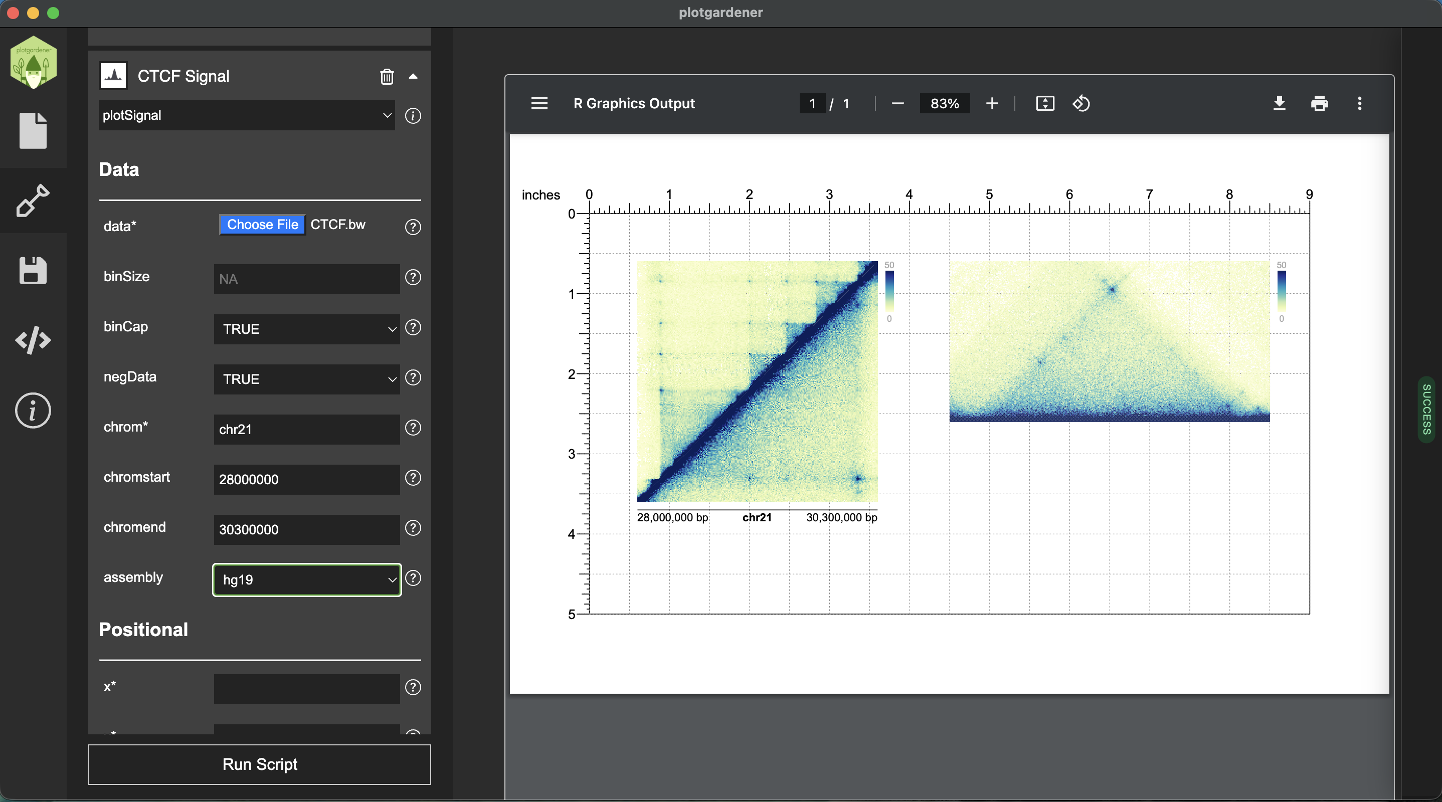
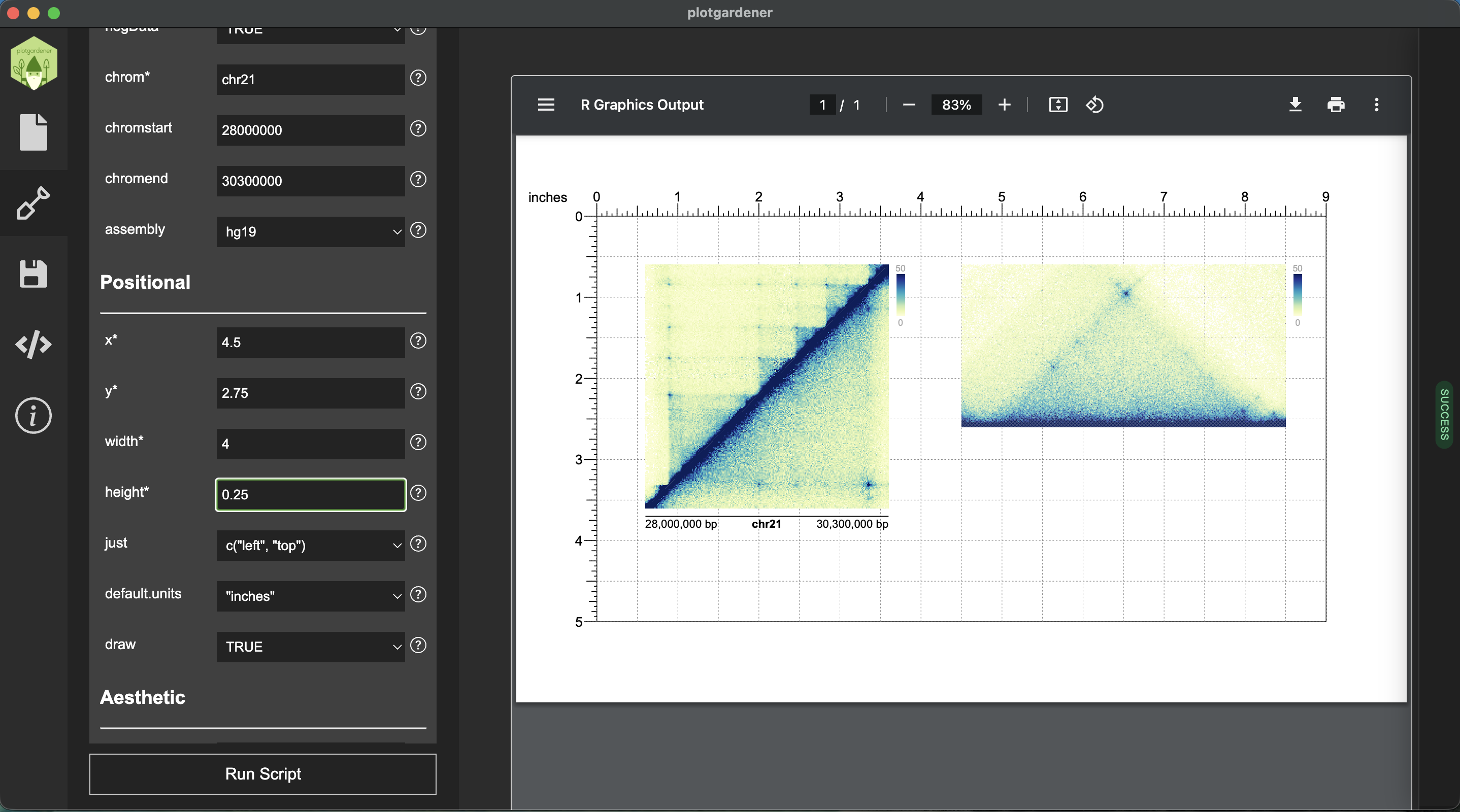
Now we will add signal tracks showing ChIP-seq data for two proteins of interest: CTCF and H3K27ac.
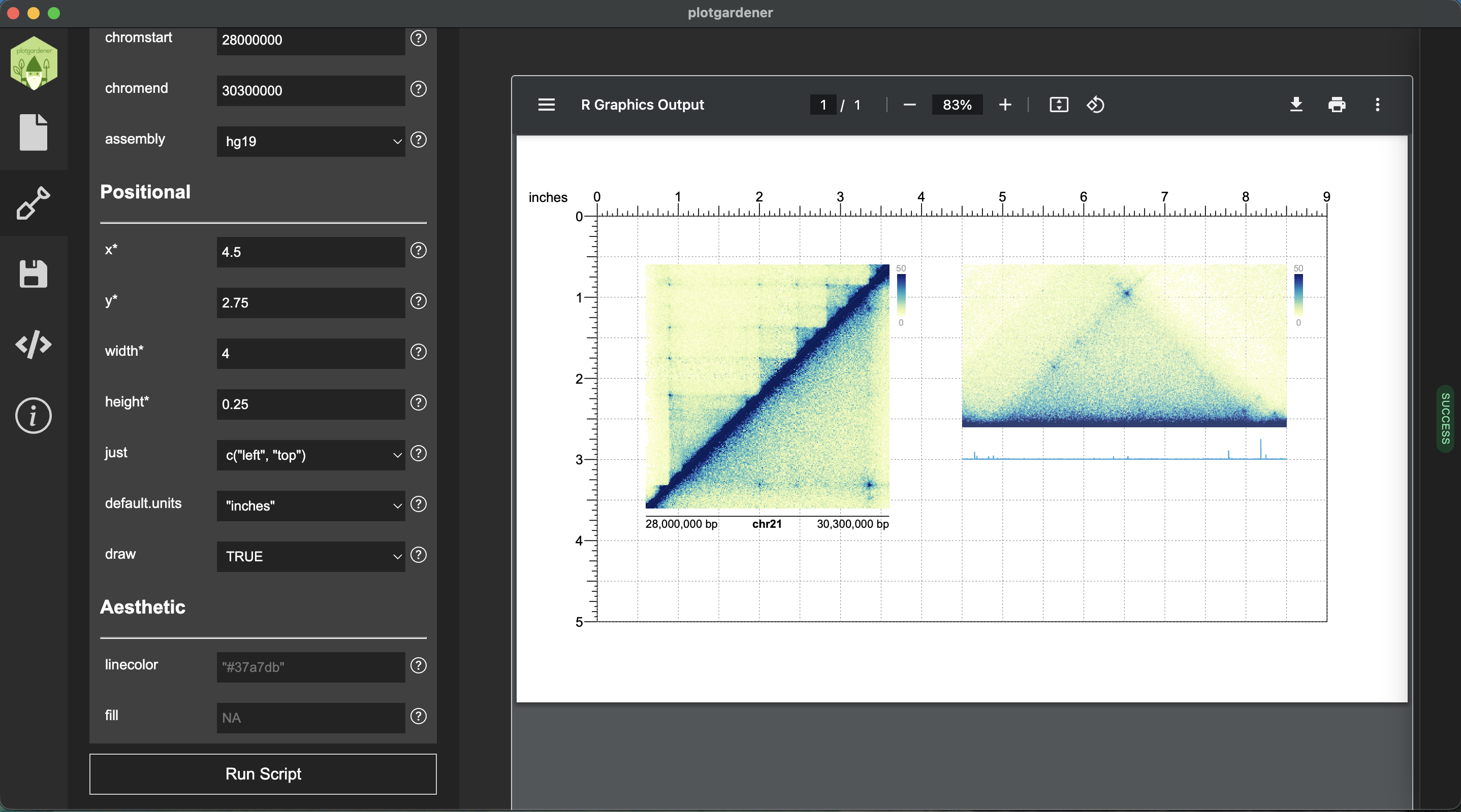
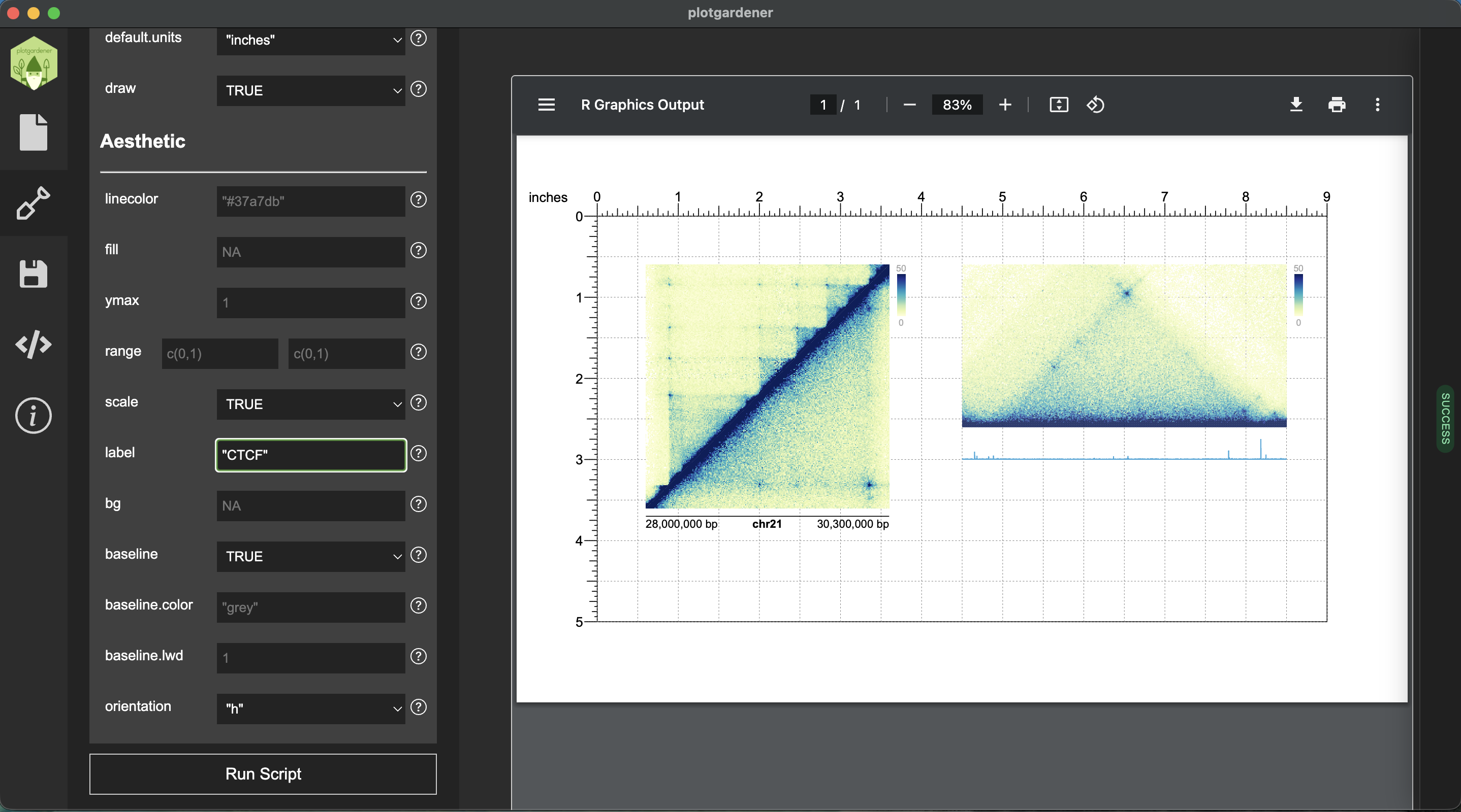
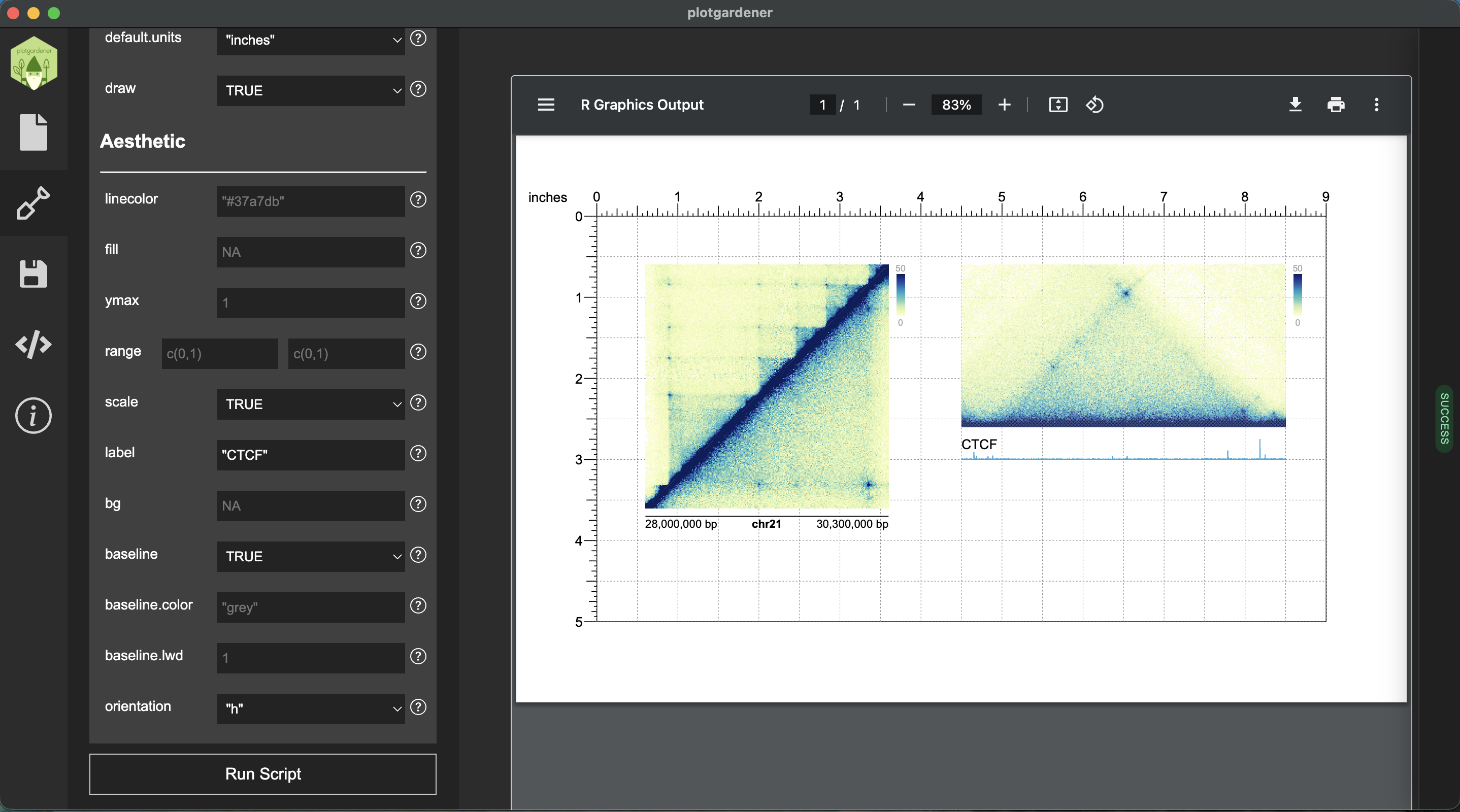
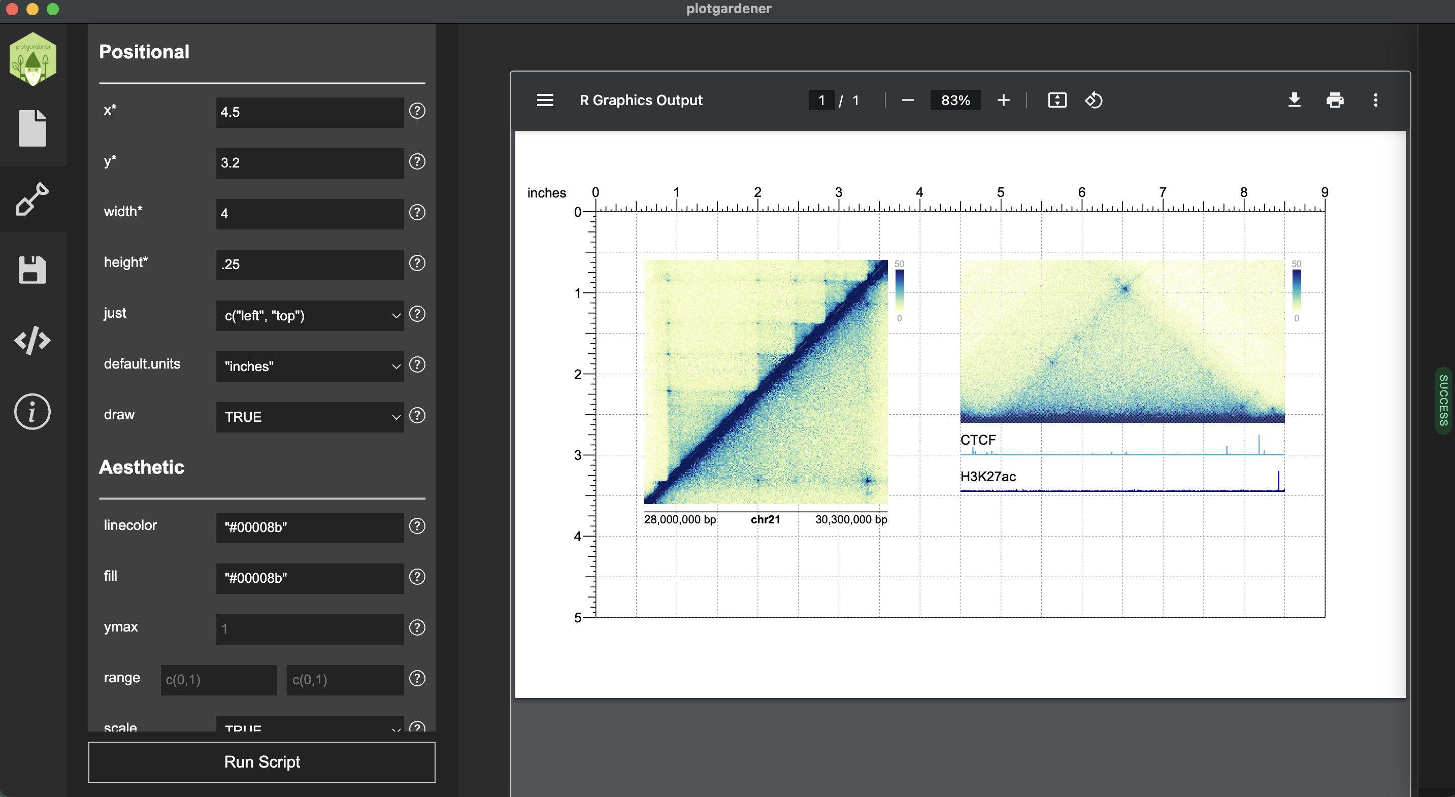
Add Gene Annotations
Click Add Plot and select plotGenes. Enter the positional parameters:
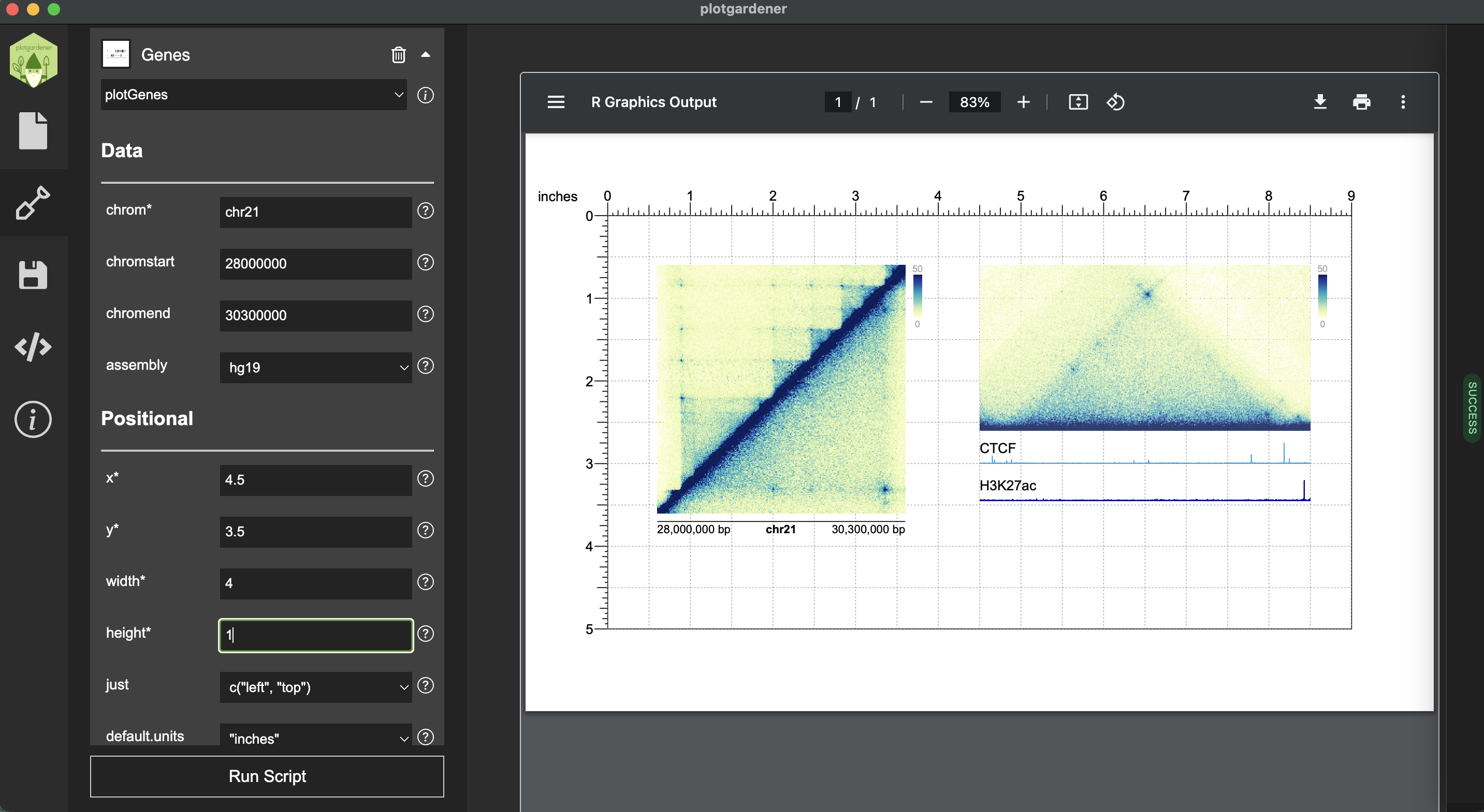
Click Run Script.
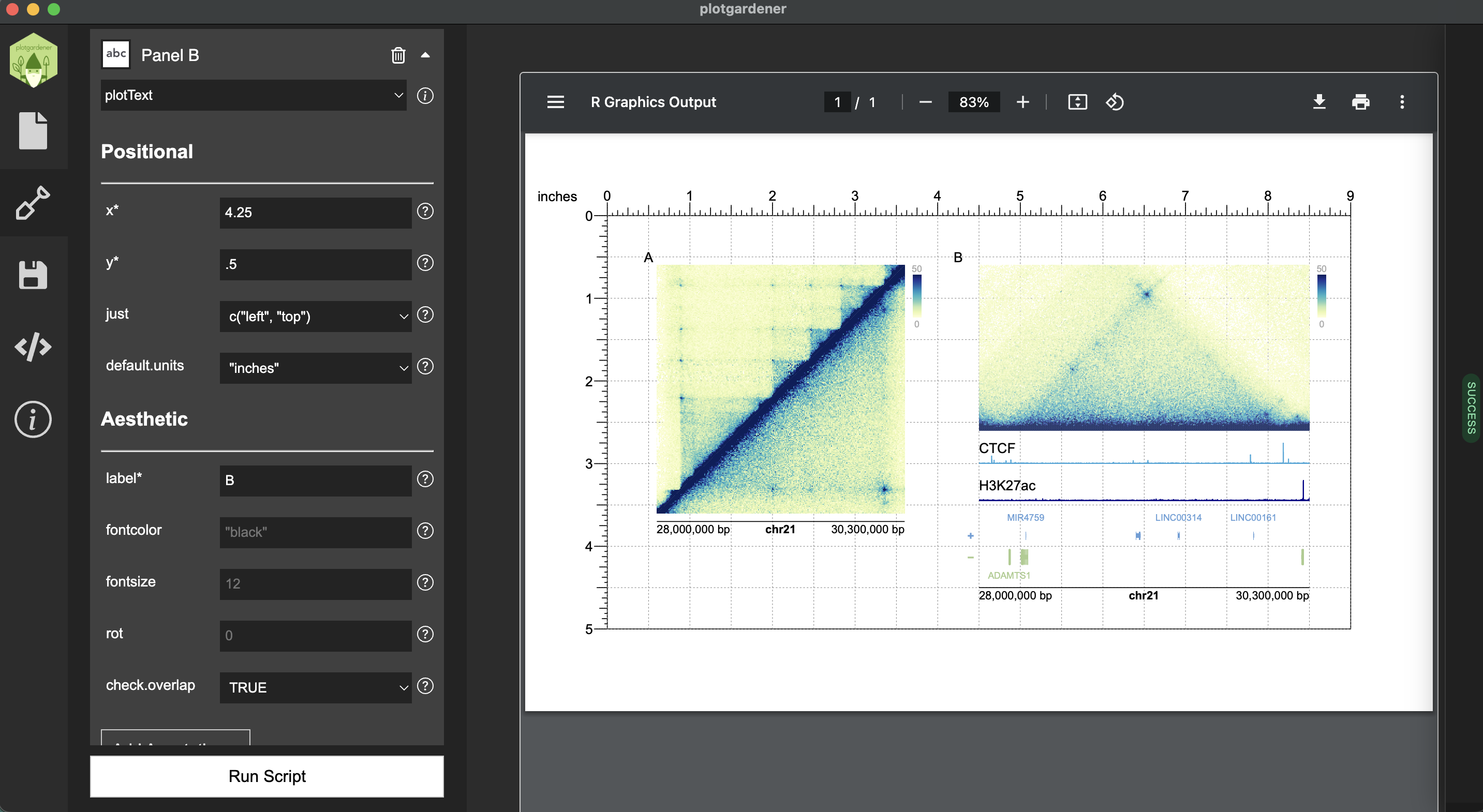
Add a Genome Label to Panel B
Return to the plotHicRectangle plot and click Add Annotation. Select annoGenomeLabel and enter the position as shown below and click Run Script.